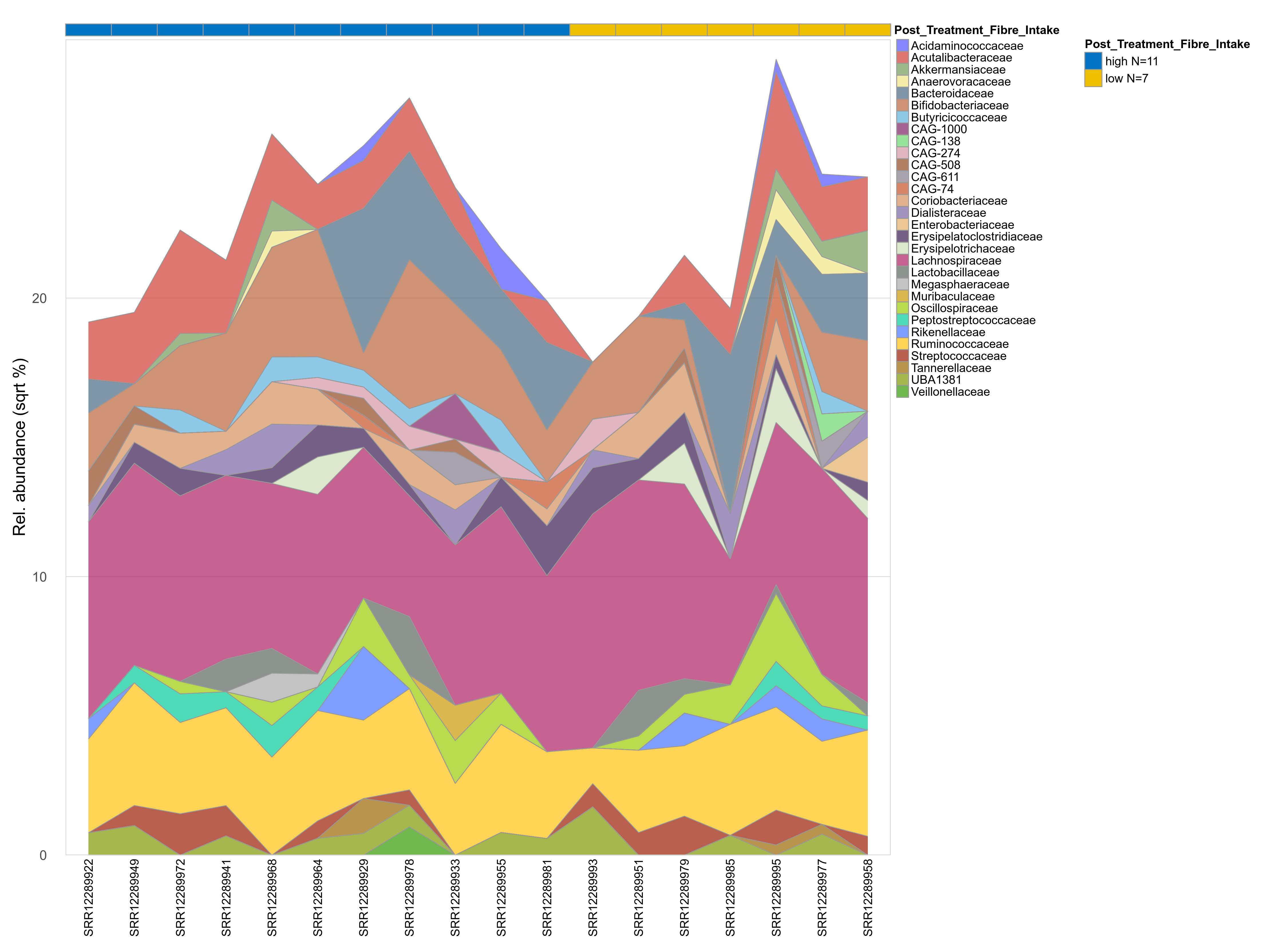
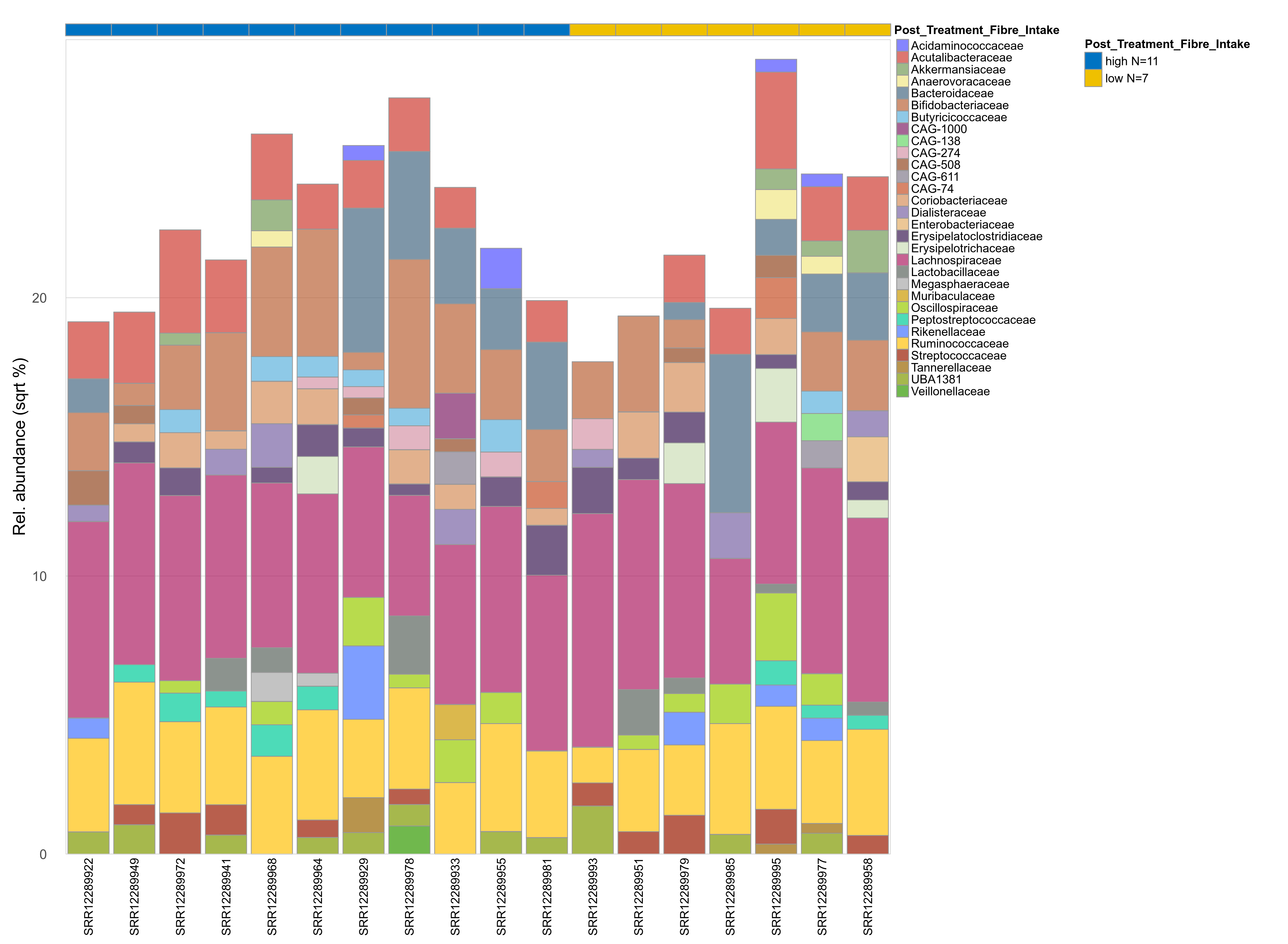
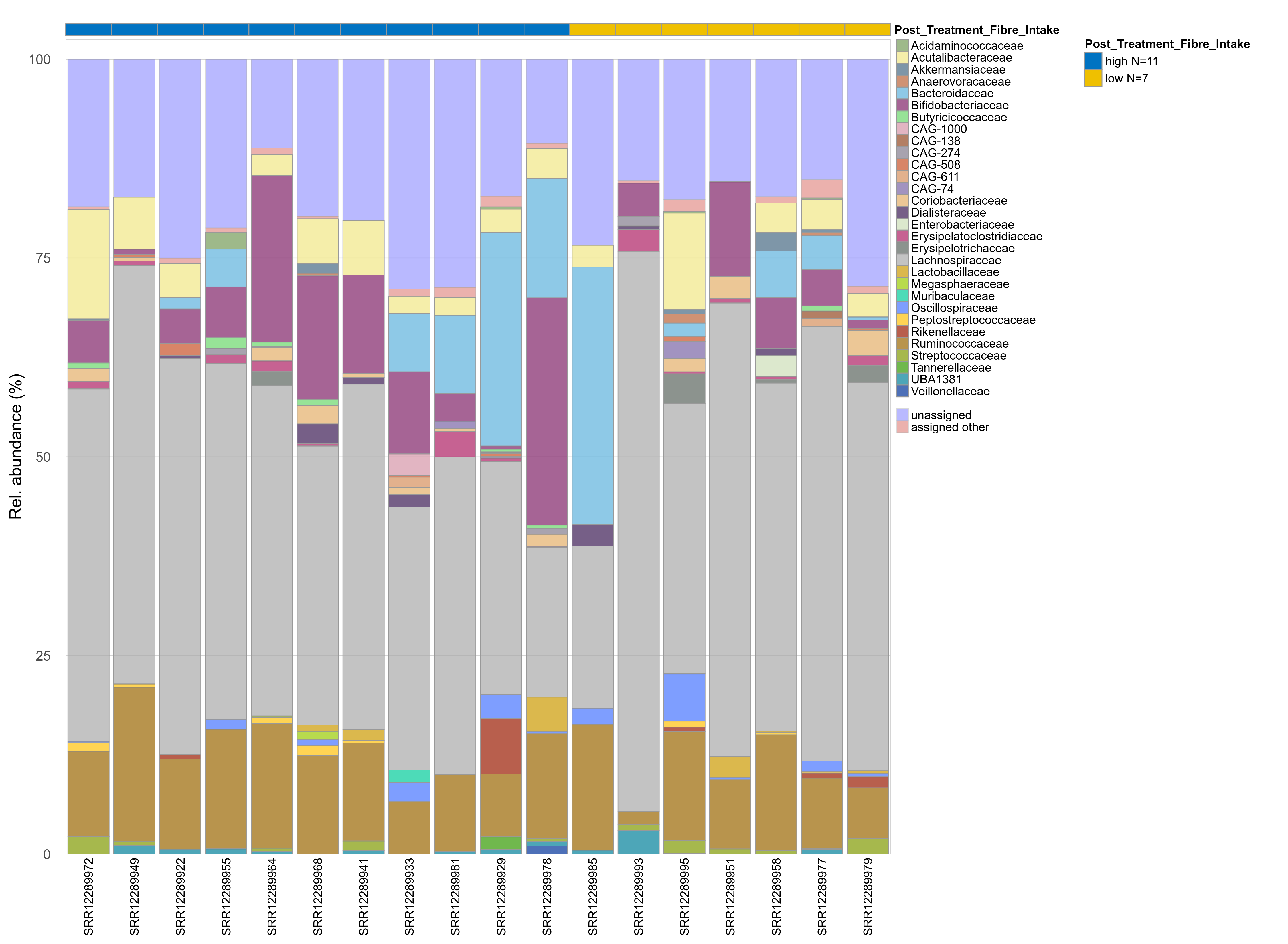
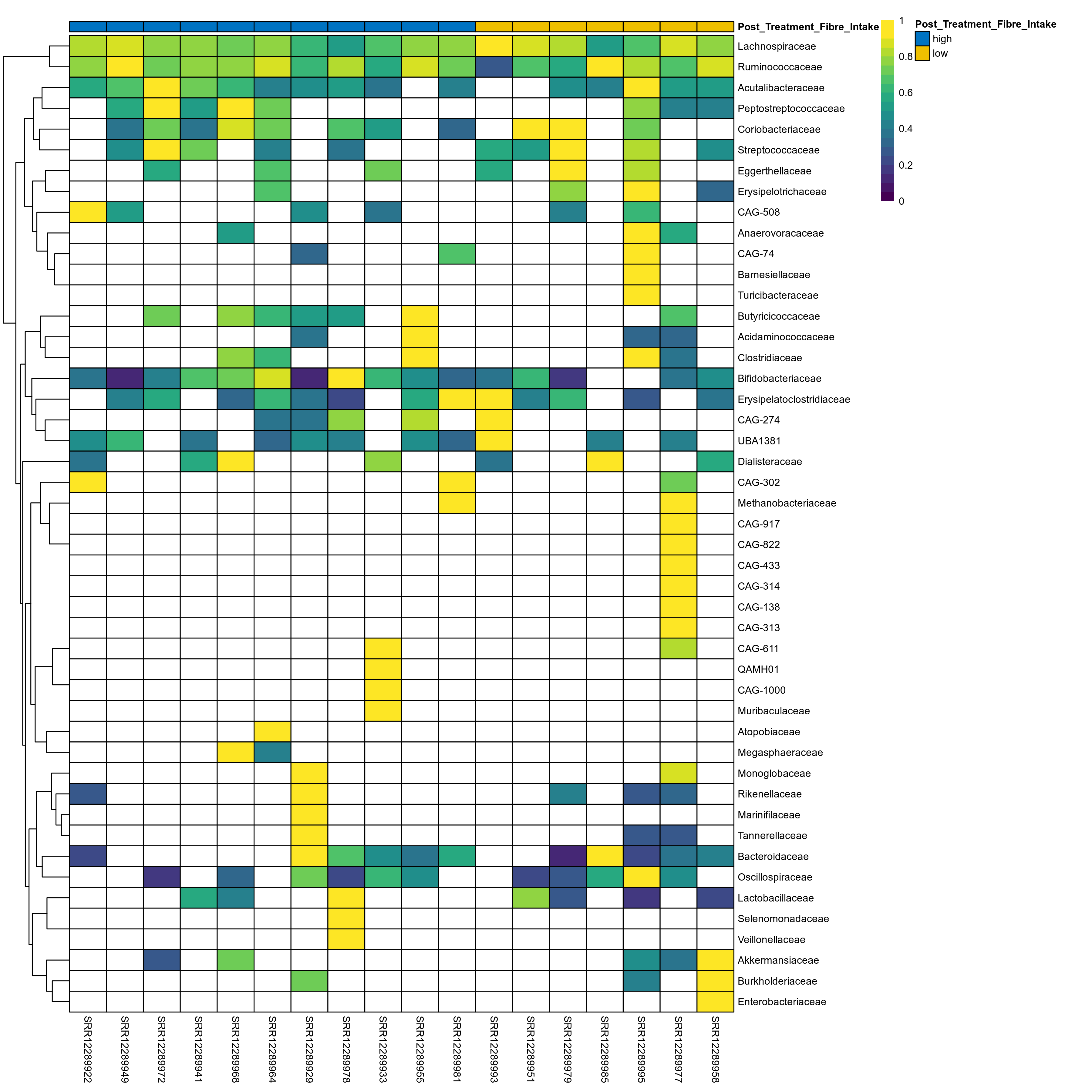
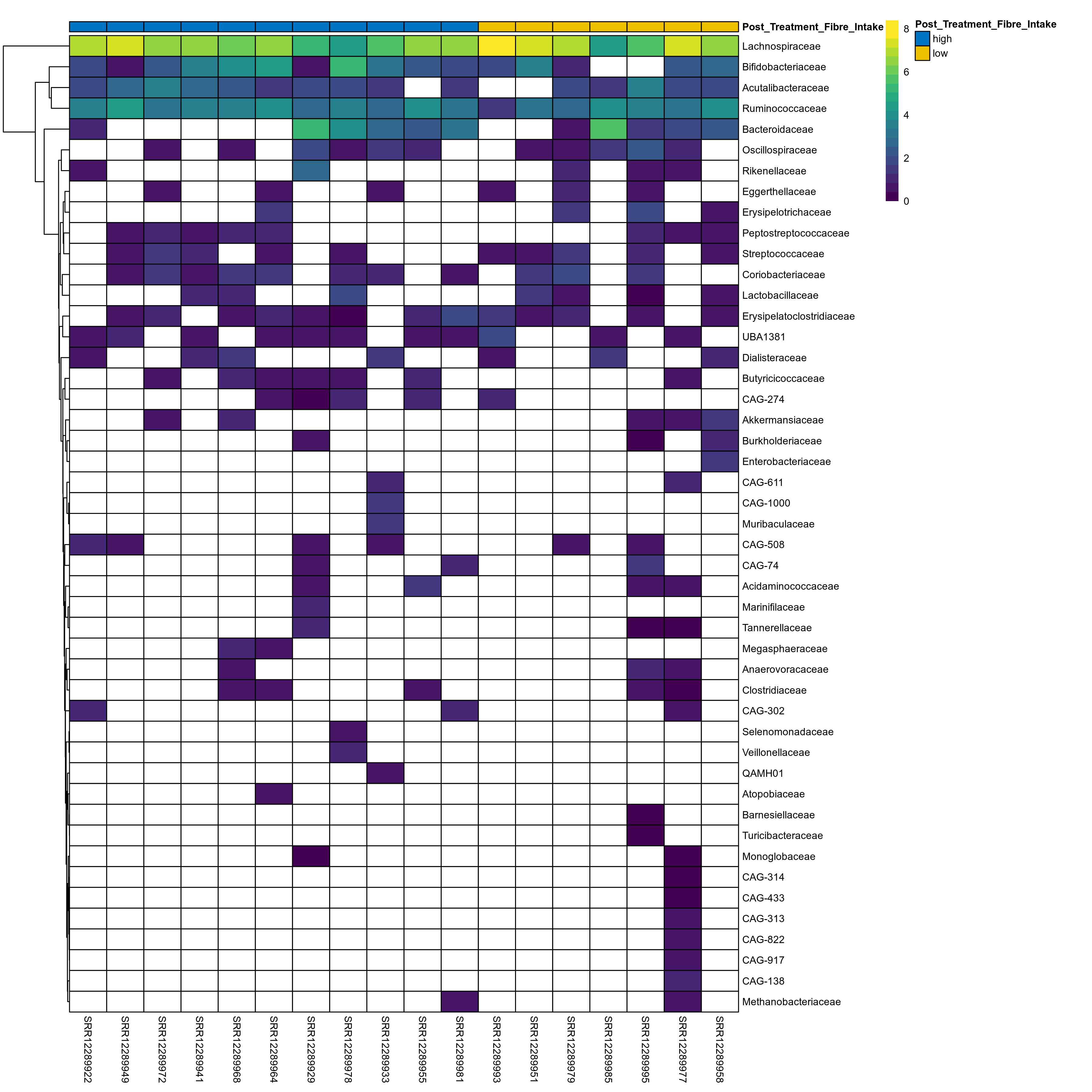
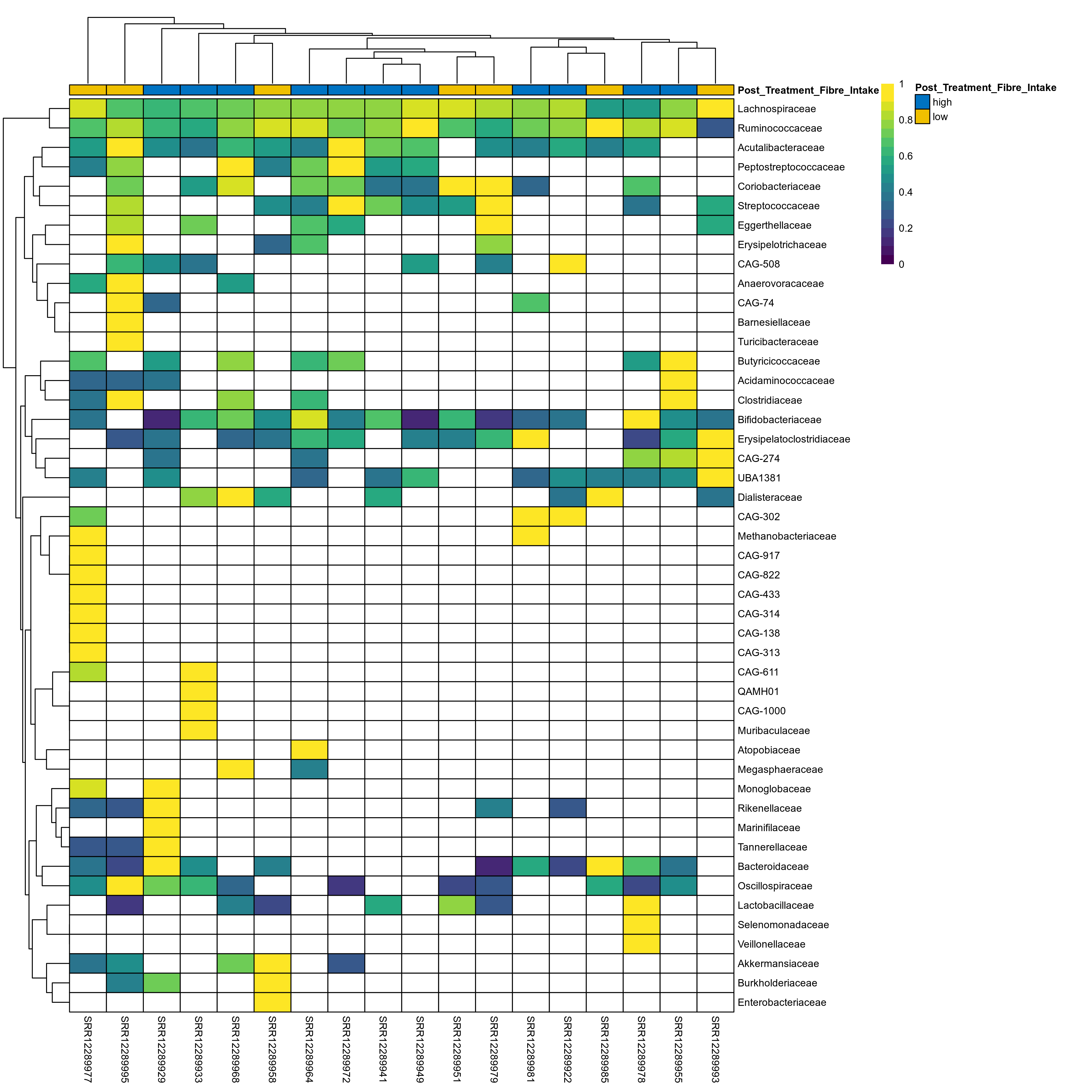
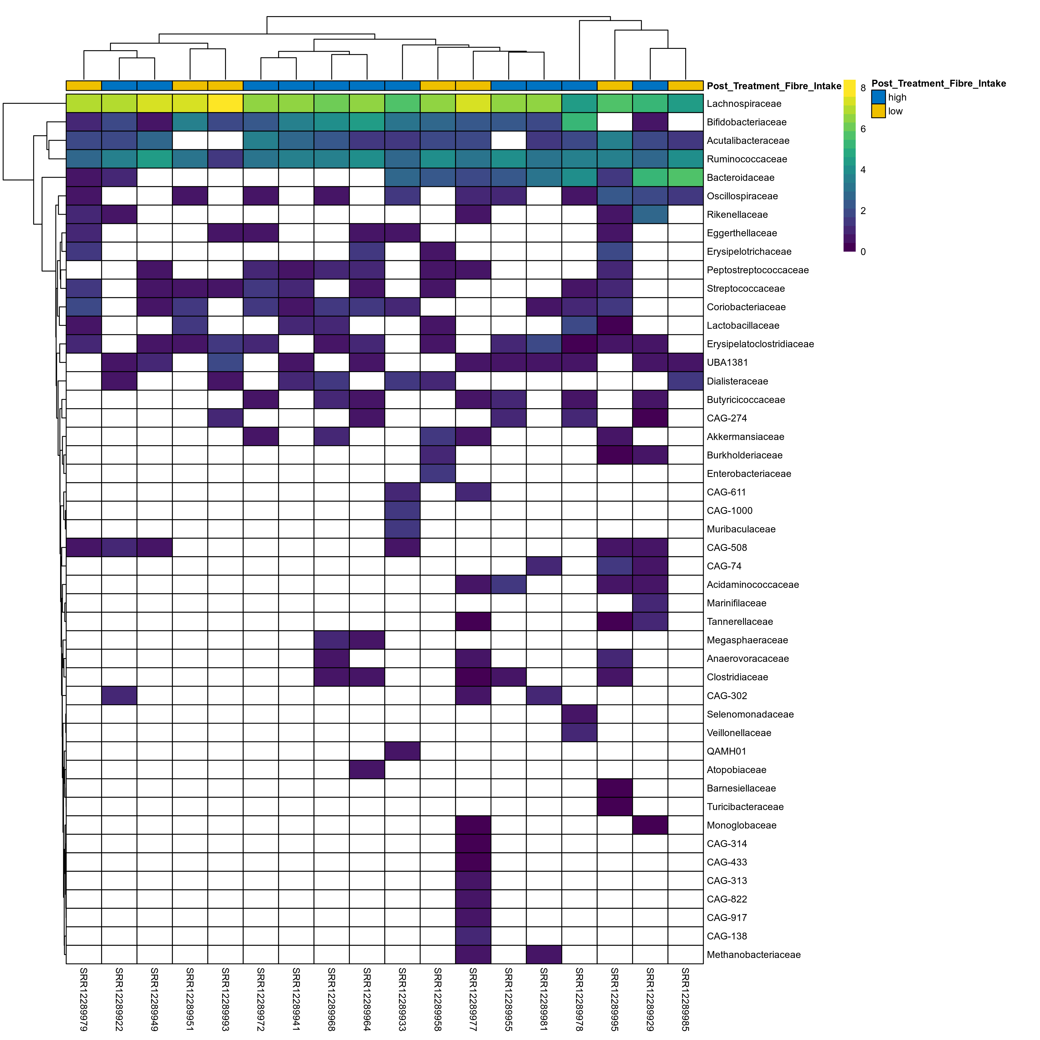
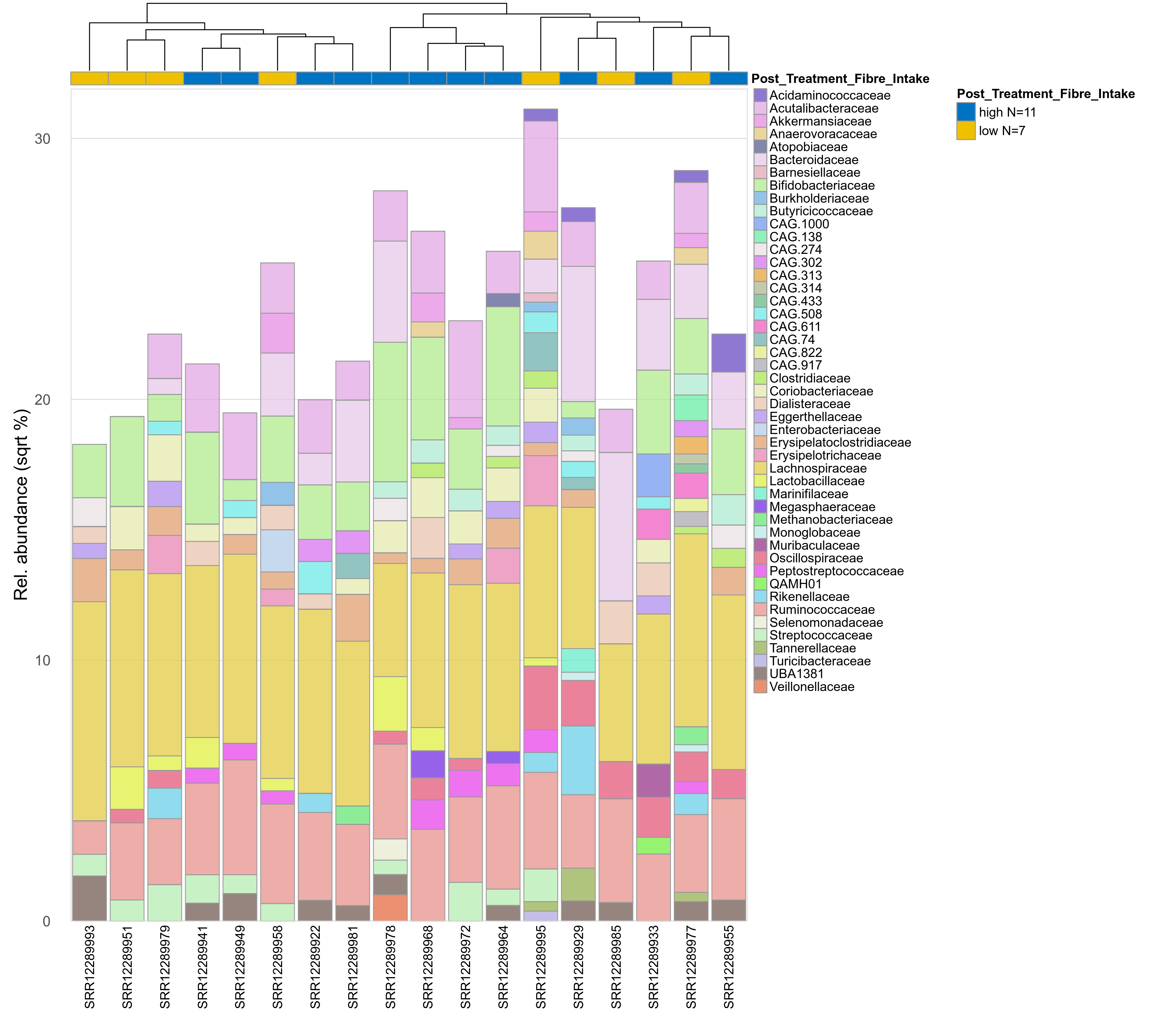
Microba Research Discovery Report

Taxonomic Profiles (Family)

The charts below show the taxonomic composition of the analysed samples using different quantitative visualization techniques. Only the top most abundant families are shown.

Areachart

Click here to open full-sized image in new window.

Barchart clustered within each group

Click here to open full-sized image in new window.

All features barchart clustered within each group

Click here to open full-sized image in new window.

Scaled heatmap of most abundant features ordered by study group

Features were filtered by mean abundance. Samples were first ordered by study group and then clustered within each study group. Abundances were scaled to a max value of 1. Color scale shows not-detected (white), and abundance ranging from low (blue) to high (yellow).

Click here to open full-sized image in new window.

Heatmap of most abundant features ordered by study group

Features were filtered by mean abundance. Samples were first ordered by study group and then clustered within each study group. Color scale shows not-detected (white), and abundance ranging from low (blue) to high (yellow).

Click here to open full-sized image in new window.

Scaled heatmap of all features

Profiles were clustered by hierarchical clustering. Abundances were scaled to a max value of 1. Color scale shows not-detected (white), and abundance ranging from low (blue) to high (yellow).

Click here to open full-sized image in new window.

Heatmap of all features

Profiles were clustered by hierarchical clustering. Color scale shows not-detected (white), and abundance ranging from low (blue) to high (yellow).

Click here to open full-sized image in new window.

Hierarchically clustered barchart

Profiles were clustered by hierarchical clustering.

Click here to open full-sized image in new window.

Interactive Barchart

Click here to open interactive barchart in new window.

Microbial alpha diversity (family)

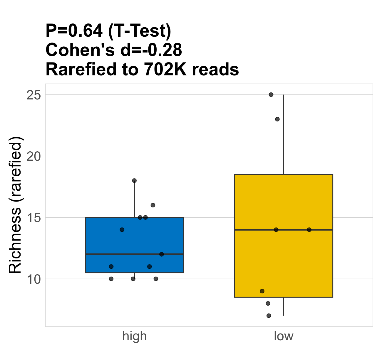
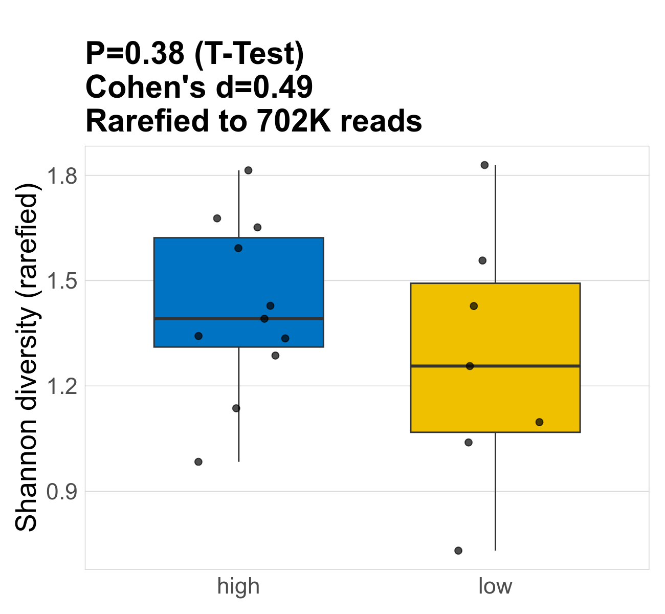
This page provides an overview of the microbial alpha diversity of the analysed samples. Alpha diversity is measured by the Shannon index and species richnes. Richness simply quantifies the total number of families present in each sample. Shannon index additionally accounts for relative abundance and evenness of the families present and quantifies the entropy of microbial communties. Barcharts and boxplots present the mean diversity in each study group.

Methods:

Shannon diversity was compared using a standard t-test. Richness was compared using a standard t-test. Data was rarefied to 702268 reads.

Index: Richness

Index: Shannon index

Summary Table

Index	rarefiedTo	P Welch's t-test	Mean Pos	Mean Abundance	Median Abundance	Mean Post_Treatment_Fibre_Intakehigh	Median Post_Treatment_Fibre_Intakehigh	SD Post_Treatment_Fibre_Intakehigh	Mean Post_Treatment_Fibre_Intakelow	Median Post_Treatment_Fibre_Intakelow	SD Post_Treatment_Fibre_Intakelow	Fold Change Log2(Post_Treatment_Fibre_Intakelow/Post_Treatment_Fibre_Intakehigh)	Positive samples	Positive Post_Treatment_Fibre_Intakehigh	Positive Post_Treatment_Fibre_Intakelow	Positive_Post_Treatment_Fibre_Intakehigh_percent	Positive_Post_Treatment_Fibre_Intakelow_percent
Shannon	702268	0.38	1.4	1.4	1.4	1.4	1.4	0.25	1.3	1.3	0.36	-0.11	18 / 18 (100%)	11 / 11 (100%)	7 / 7 (100%)	1	1
Richness	702268	0.64	13	13	13	13	12	2.8	14	14	7.2	0.11	18 / 18 (100%)	11 / 11 (100%)	7 / 7 (100%)	1	1

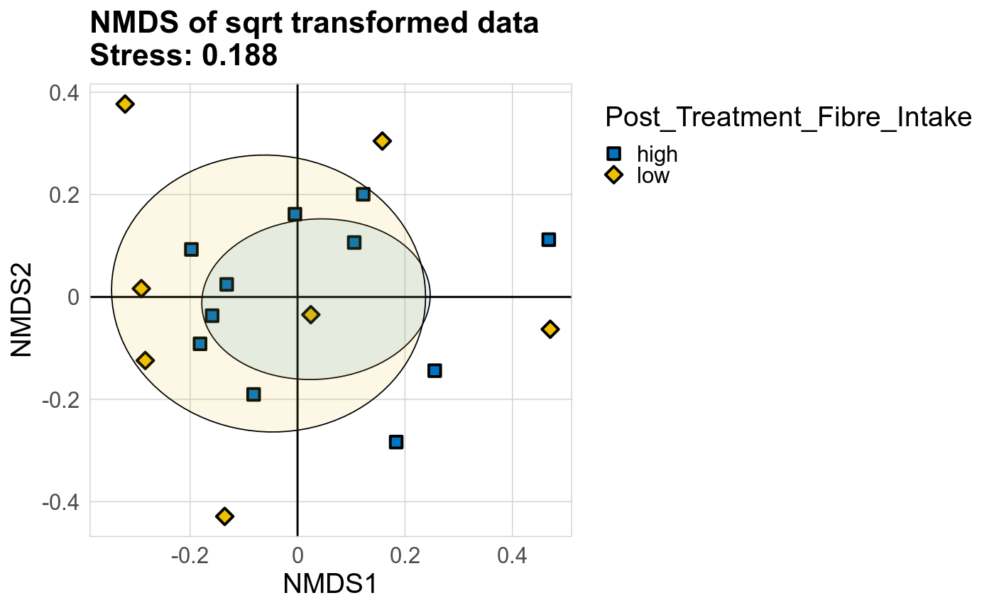
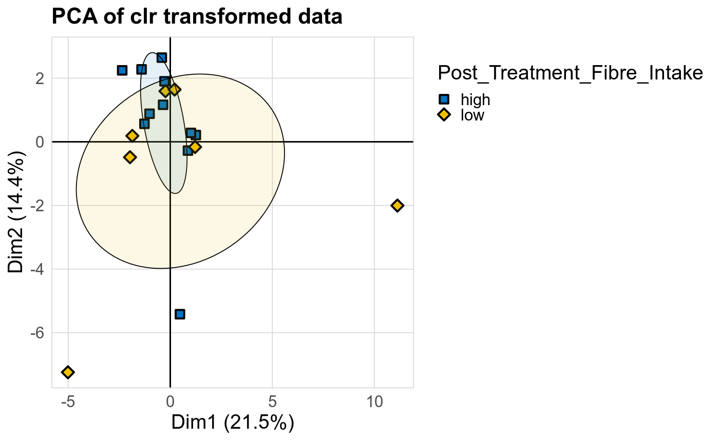
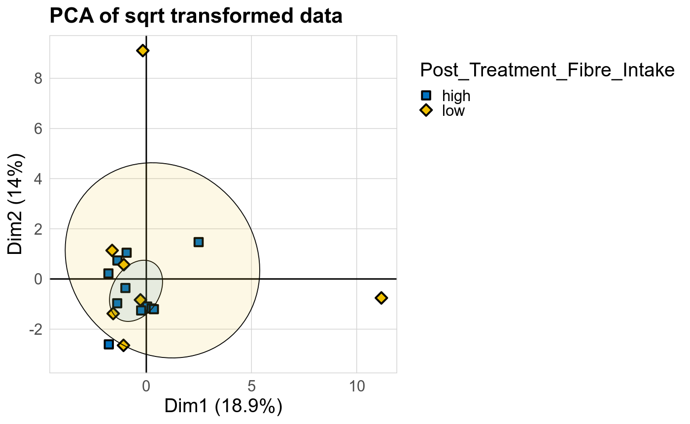
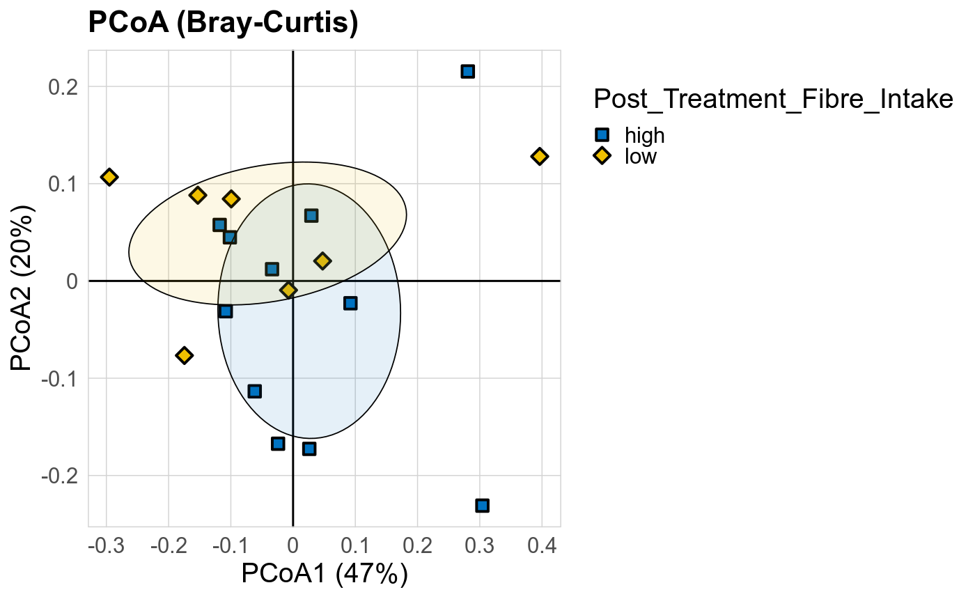
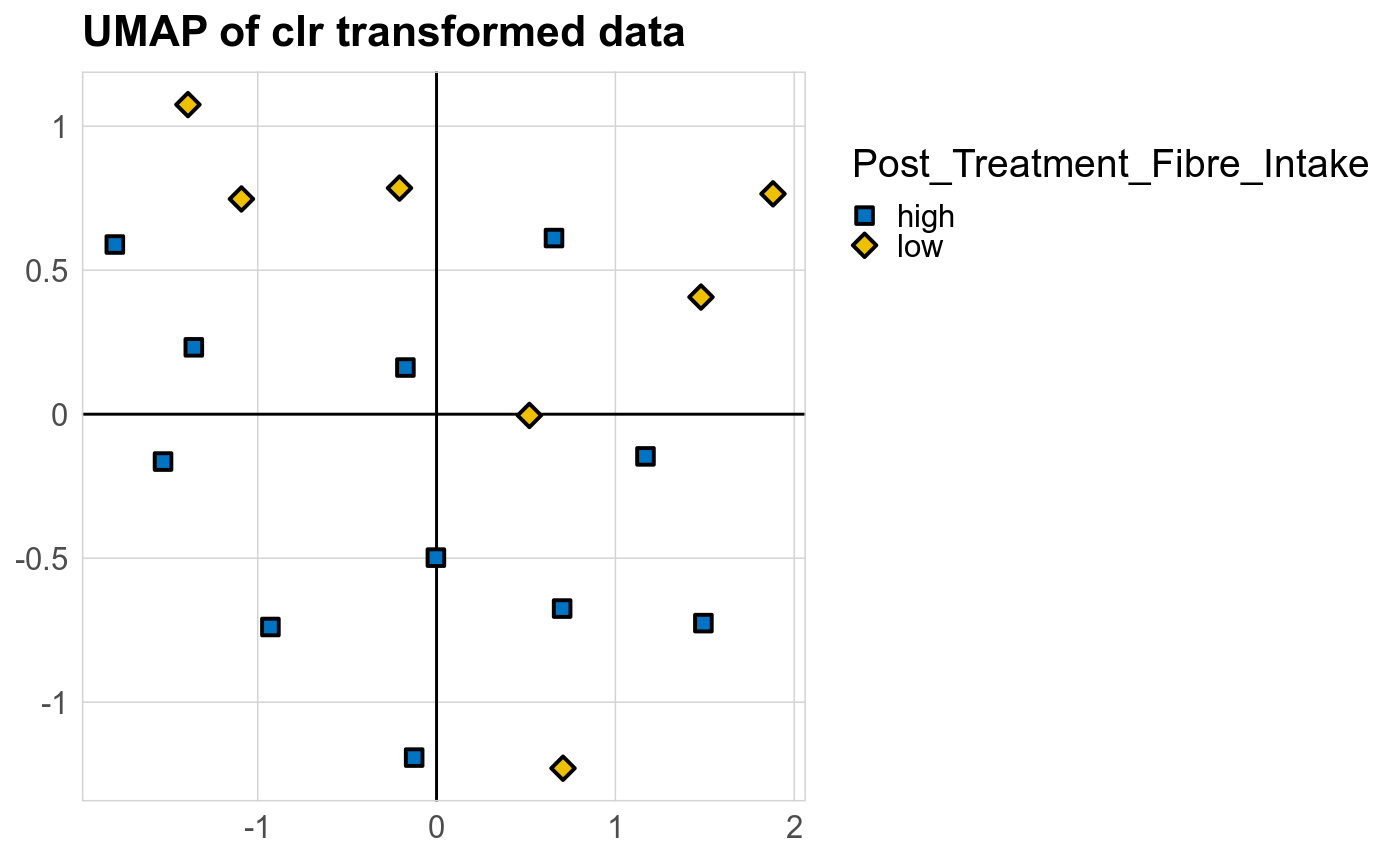
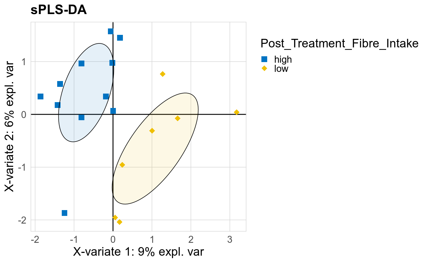
Download diversity values in csv format . On some platforms (including Windows) you may need to change the suffix from .txt or .html to .csv before opening the file in a spreadsheet program, like Excel.

Clustering and ordination (family)

Taxonomic profiles were analyzed using supervised and unsupervised multivariate methods. Profiles were ordinated using the unsupervised methods Principal Coordinates Analysis (PCoA), Non-Metric Multidimensional Scaling (NMDS) and Principal Component Analysis (PCA). PCoA and NMDS are related to PCA, but take dissimlarity matrices as input. PCoA and NMDS both attempt to represent the pairwise dissimlarities between samples in low dimensional space as close as possible. NMDS is a rank-based approach and therefore less effected by outliers.

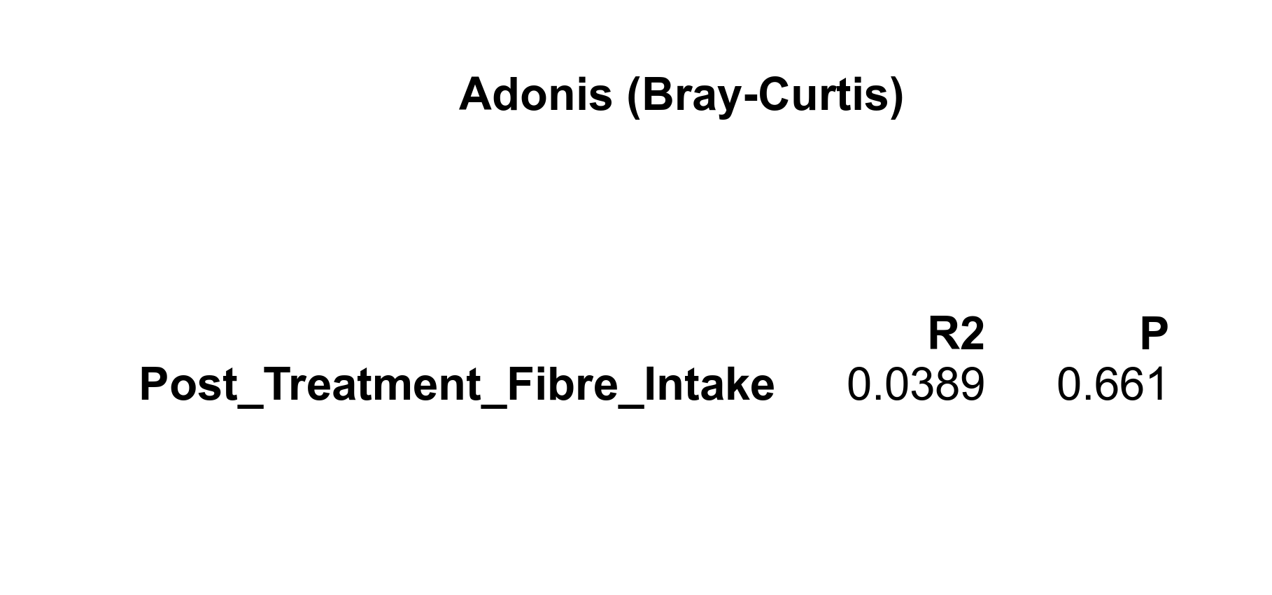
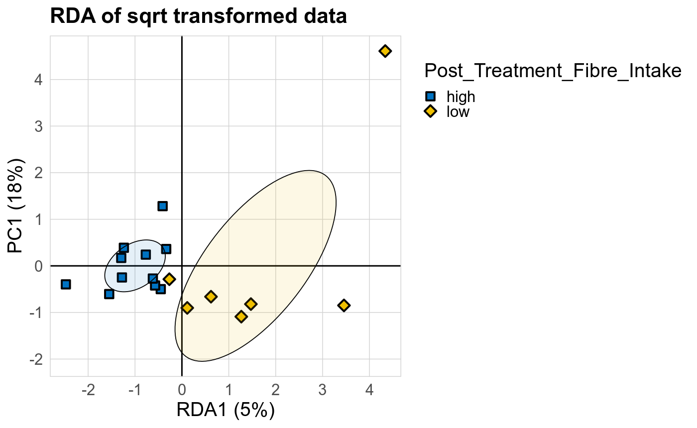
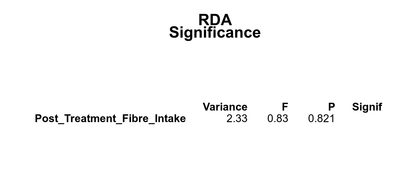
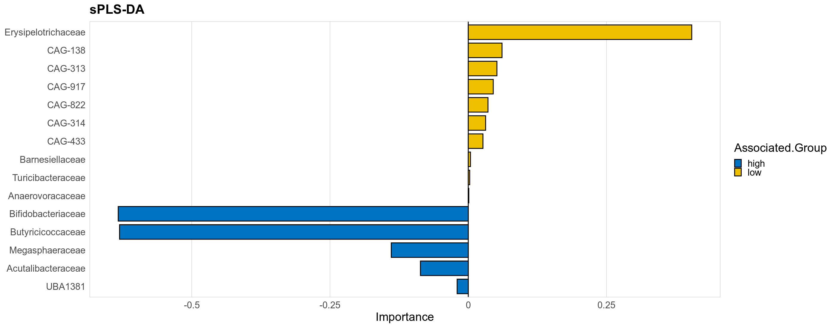
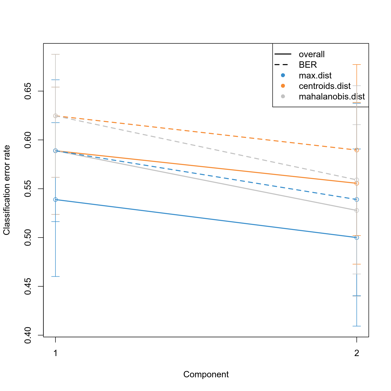
The supervised methods Adonis and Redundancy analysis (RDA) were used to assess if variance in microbial community composition can be attributed to the study condition. NMDS, PCoA and Adonis were run on Bray-Curtis dissimilarities. A short introduction of the used methods can be found at the GUide to STatistical Analysis in Microbial Ecology (GUSTA ME). Sparse Partial Least Square Discriminant Analysis (sPLS-DA) from the MixMc package was additionaly used to extract features associated with the study condition.

Unsupervised ordination

Interactive PCA (clr transformed)

Please click here to view an interactive 3D PCoA.

Please click here to view an interactive 3D PCA.

Supervised Analysis

sPLS-DA

Univariate analysis of family abundance

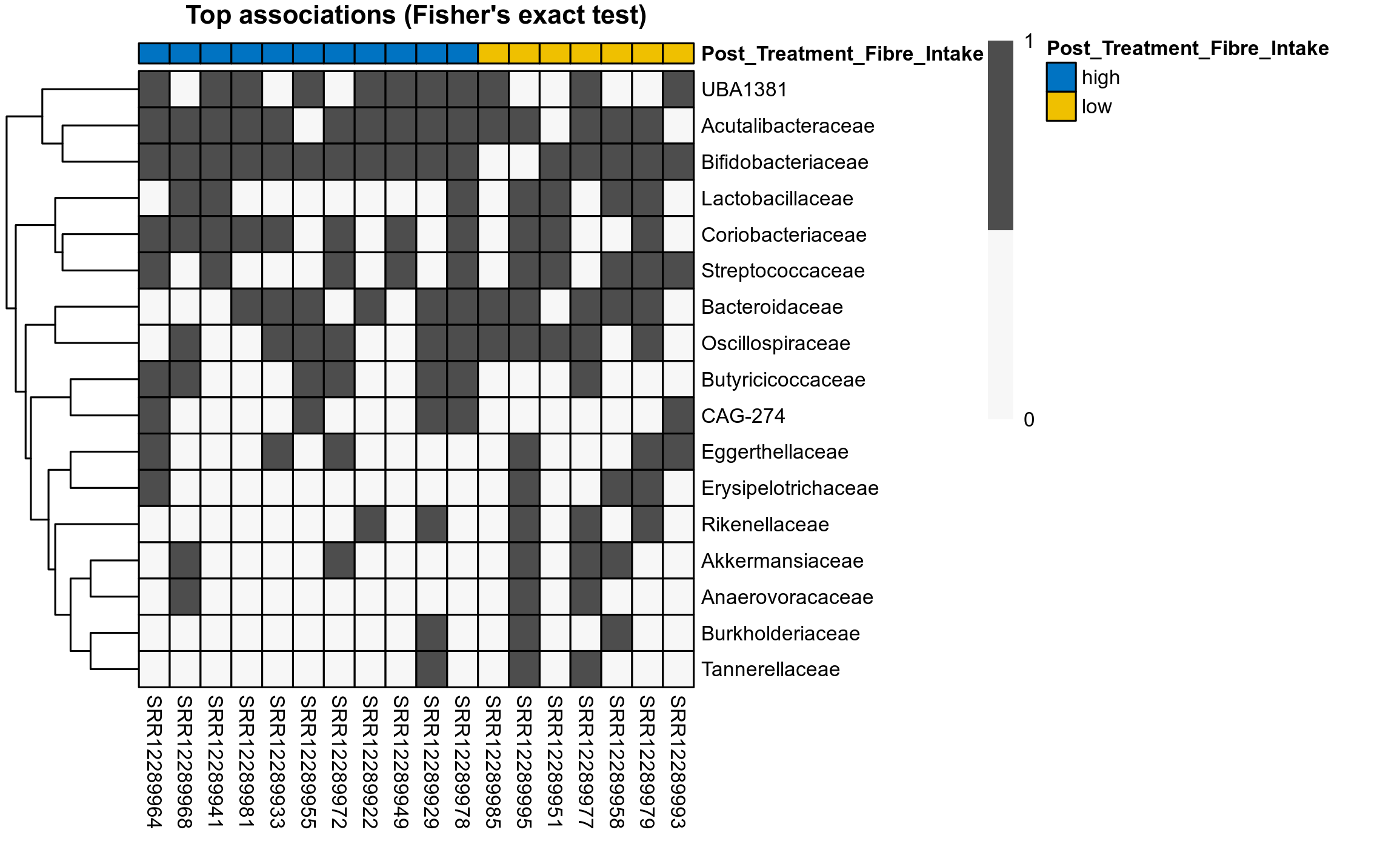
Differentially abundant families were identified by ANOVA or LMER (linear mixed effect regression) of clr transformed relative abudances, Fisher's exact test and/or ALDEx2 (on families read counts). Fisher's exact test is used to test for differences in the detection rate, i.e. number of samples in which each family has been detected.

LMER is used for repeated measures data, using random effects to control for correlation between samples from the same subject. Fixed effects are included for treatment groups, time, and treatment over time, where appropriate. The LMER P values correspond to a nested model test of the significance of including the corresponding fixed effect.

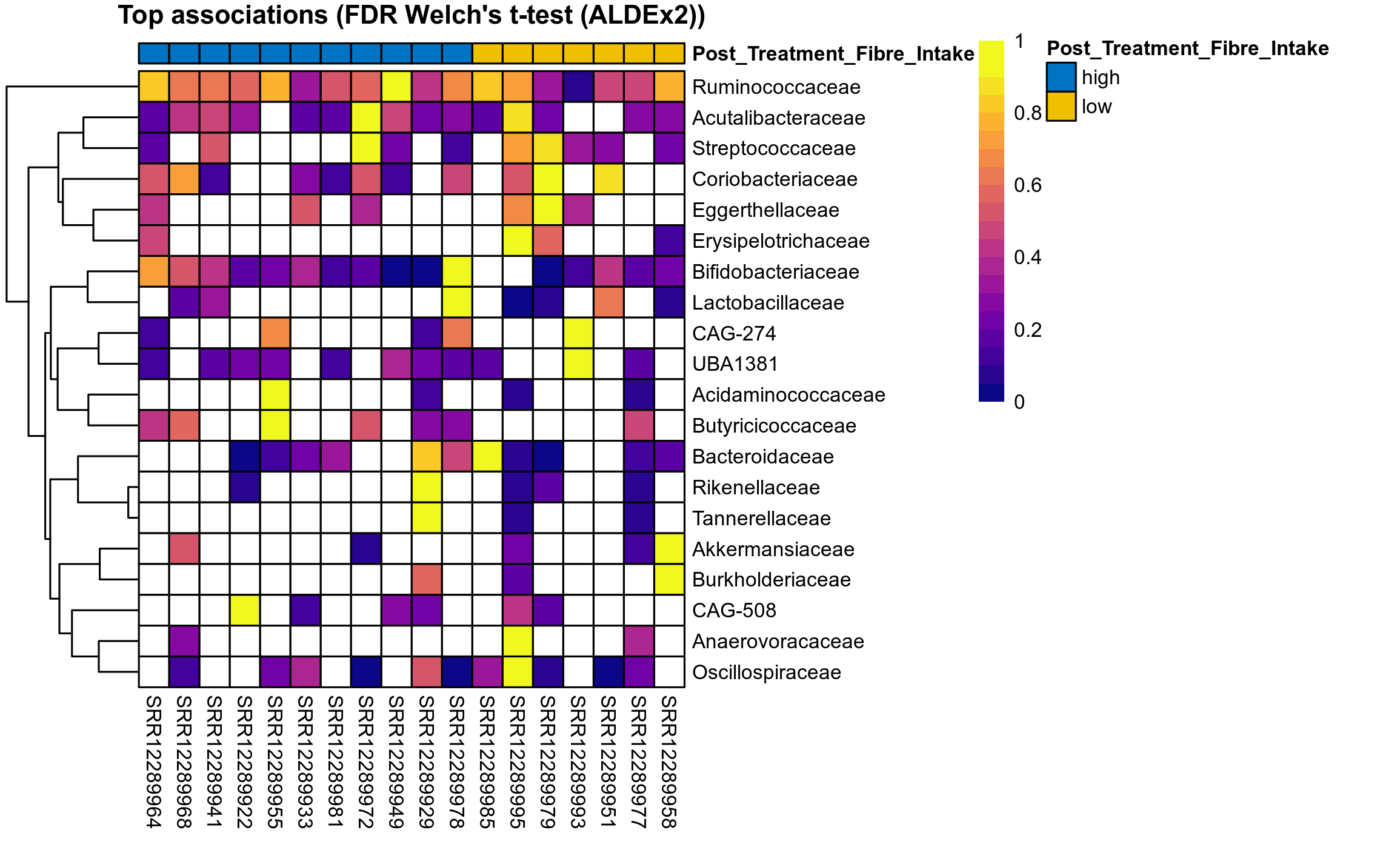
ALDEx2 uses subsampling (Bayesian sampling) to estimate the underlying technical variation. For each subsample instance, center log-ratio transformed data is statistically compared across study groups and computed P values are corrected for multiple testing using the Benjamini–Hochberg procedure. The expected P value (mean P value) is reported, which are those that would likely have been observed if the same samples had been run multiple times. The expected values are reported for both the distribution of P values and for the distribution of Benjamini–Hochberg corrected values.

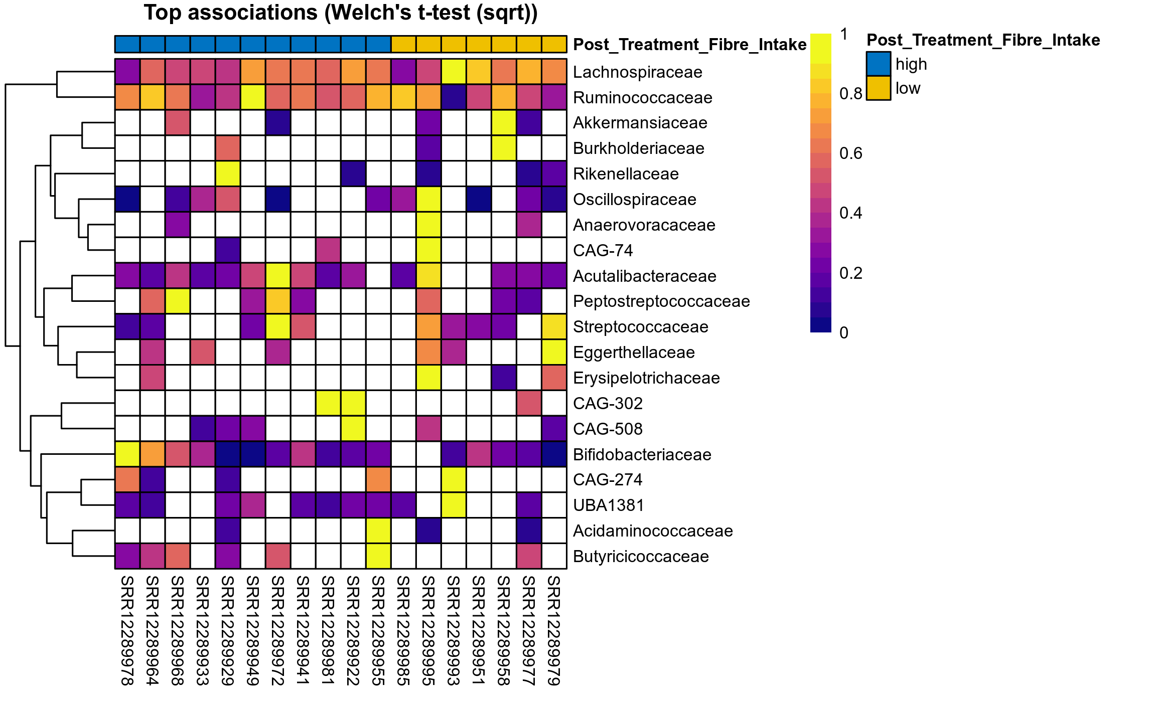
Taxon	GTDB taxonomy	P Welch's t-test (sqrt)	FDR Welch's t-test (sqrt)	Pbonf Welch's t-test (sqrt)	Cohen's d Welch's t-test (sqrt)	P Welch's t-test (clr)	FDR Welch's t-test (clr)	Pbonf Welch's t-test (clr)	Cohen's d Welch's t-test (clr)	P Fisher's exact test	FDR Fisher's exact test	Pbonf Fisher's exact test	P Welch's t-test (ALDEx2)	FDR Welch's t-test (ALDEx2)	P Wilcoxon rank test (ALDEx2)	FDR Wilcoxon rank test (ALDEx2)	Mean Pos	Mean Abundance	Median Abundance	Mean Post_Treatment_Fibre_Intakehigh	Median Post_Treatment_Fibre_Intakehigh	SD Post_Treatment_Fibre_Intakehigh	Mean Post_Treatment_Fibre_Intakelow	Median Post_Treatment_Fibre_Intakelow	SD Post_Treatment_Fibre_Intakelow	Fold Change Log2(Post_Treatment_Fibre_Intakelow/Post_Treatment_Fibre_Intakehigh)	Positive samples	Positive Post_Treatment_Fibre_Intakehigh	Positive Post_Treatment_Fibre_Intakelow	Positive_Post_Treatment_Fibre_Intakehigh_percent	Positive_Post_Treatment_Fibre_Intakelow_percent
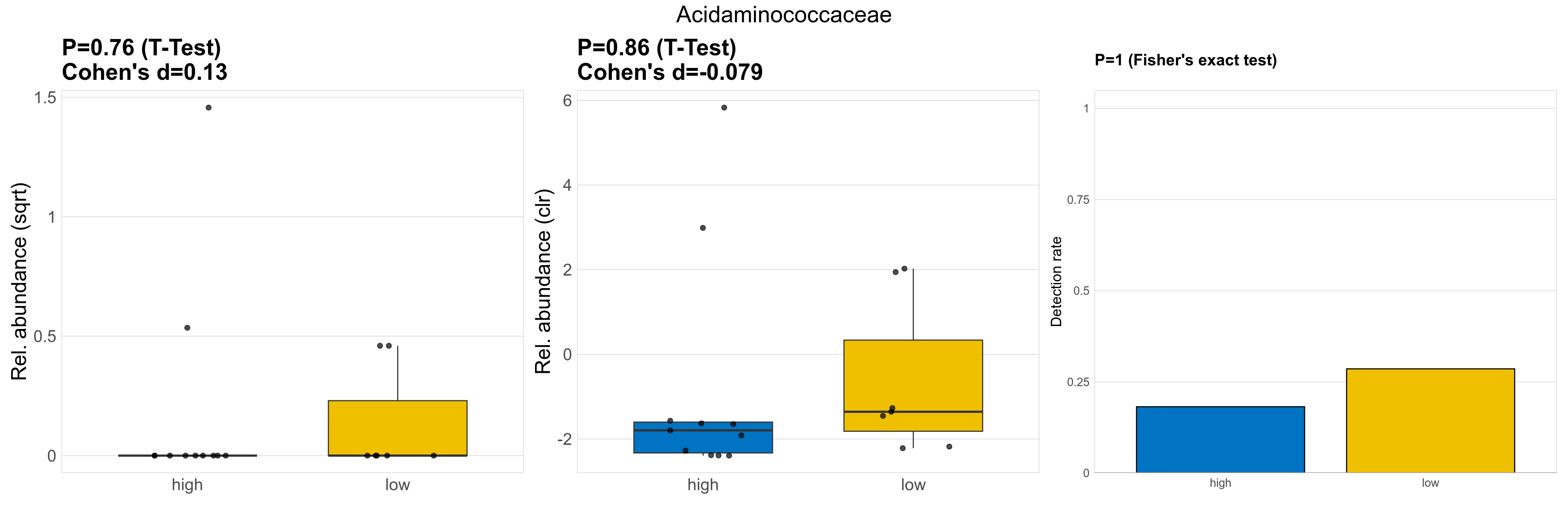
Acidaminococcaceae	Acidaminococcaceae	0.76	0.98	1	0.13	0.86	0.95	1	-0.079	1	1	1	0.69	0.87	0.56	0.88	0.71	0.16	0	0.22	0	0.64	0.06	0	0.1	-1.9	4 / 18 (22%)	2 / 11 (18%)	2 / 7 (29%)	0.182	0.286
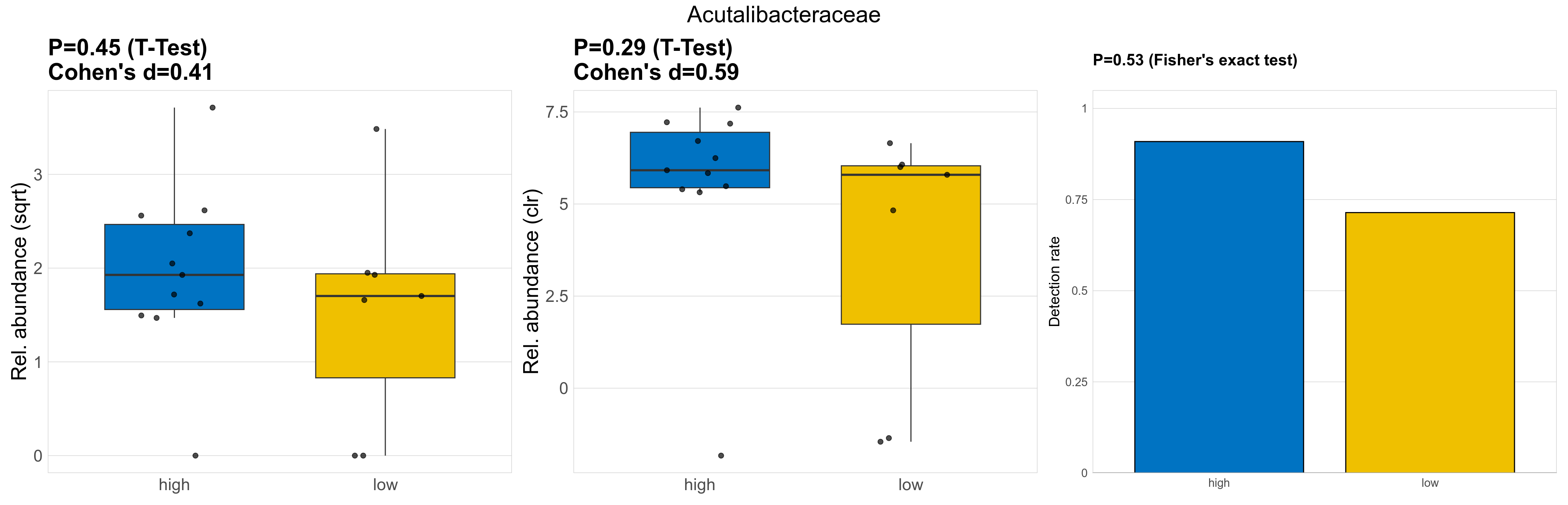
Acutalibacteraceae	Acutalibacteraceae	0.45	0.98	1	0.41	0.29	0.85	1	0.59	0.53	0.94	1	0.26	0.76	0.095	0.7	5.1	4.2	3.3	4.6	3.7	3.7	3.6	2.9	4.1	-0.35	15 / 18 (83%)	10 / 11 (91%)	5 / 7 (71%)	0.909	0.714
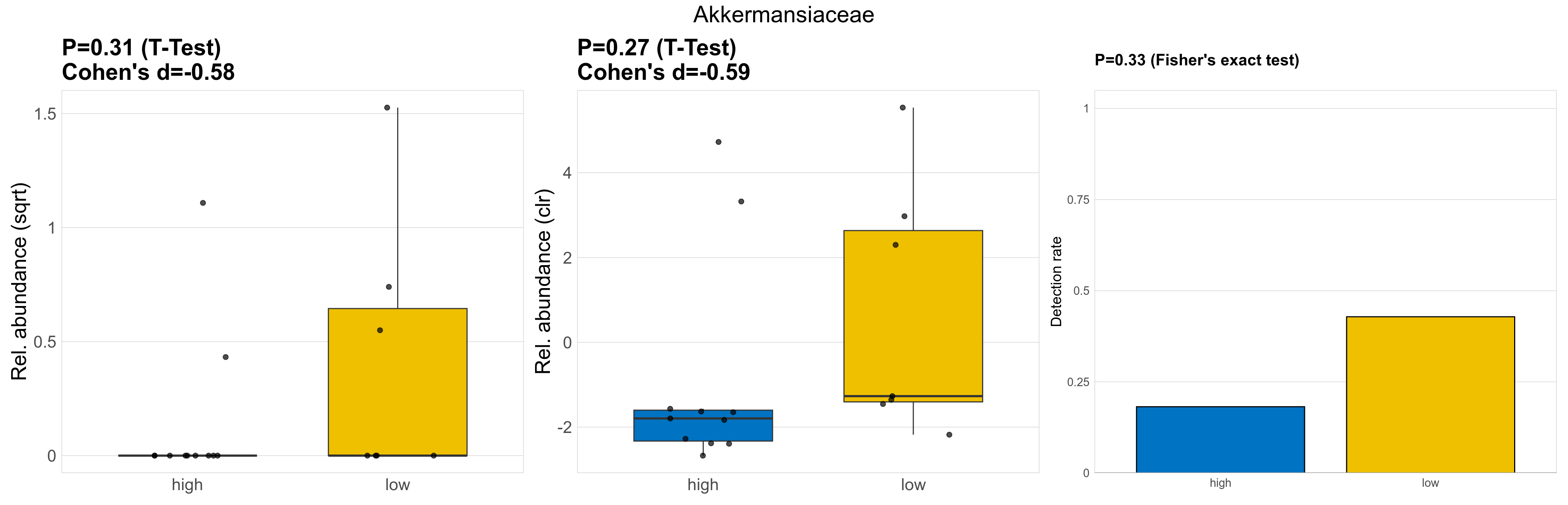
Akkermansiaceae	Akkermansiaceae	0.31	0.98	1	-0.58	0.27	0.85	1	-0.59	0.33	0.94	1	0.28	0.78	0.3	0.77	0.92	0.26	0	0.13	0	0.37	0.45	0	0.85	1.8	5 / 18 (28%)	2 / 11 (18%)	3 / 7 (43%)	0.182	0.429
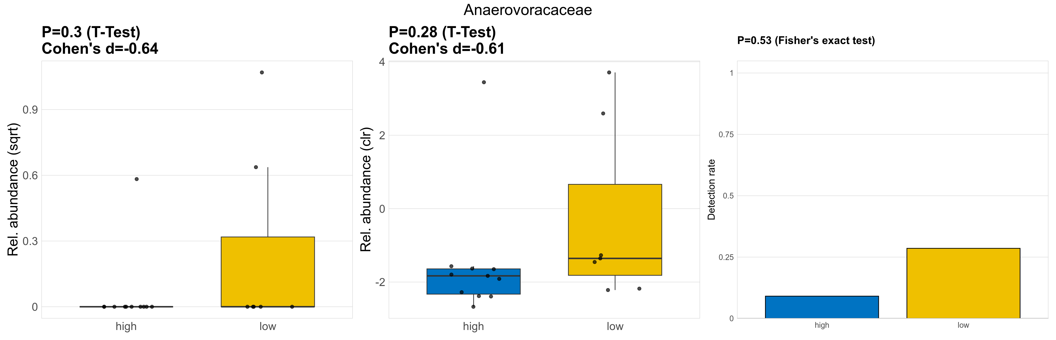
Anaerovoracaceae	Anaerovoracaceae	0.3	0.98	1	-0.64	0.28	0.85	1	-0.61	0.53	0.94	1	0.3	0.77	0.31	0.77	0.63	0.1	0	0.031	0	0.1	0.22	0	0.43	2.8	3 / 18 (17%)	1 / 11 (9.1%)	2 / 7 (29%)	0.0909	0.286
Bacteroidaceae	Bacteroidaceae	0.95	0.98	1	-0.033	0.69	0.89	1	-0.19	0.64	0.94	1	0.62	0.87	0.89	0.97	10	6.1	1.6	5.9	1.5	8.6	6.4	1.7	12	0.12	11 / 18 (61%)	6 / 11 (55%)	5 / 7 (71%)	0.545	0.714
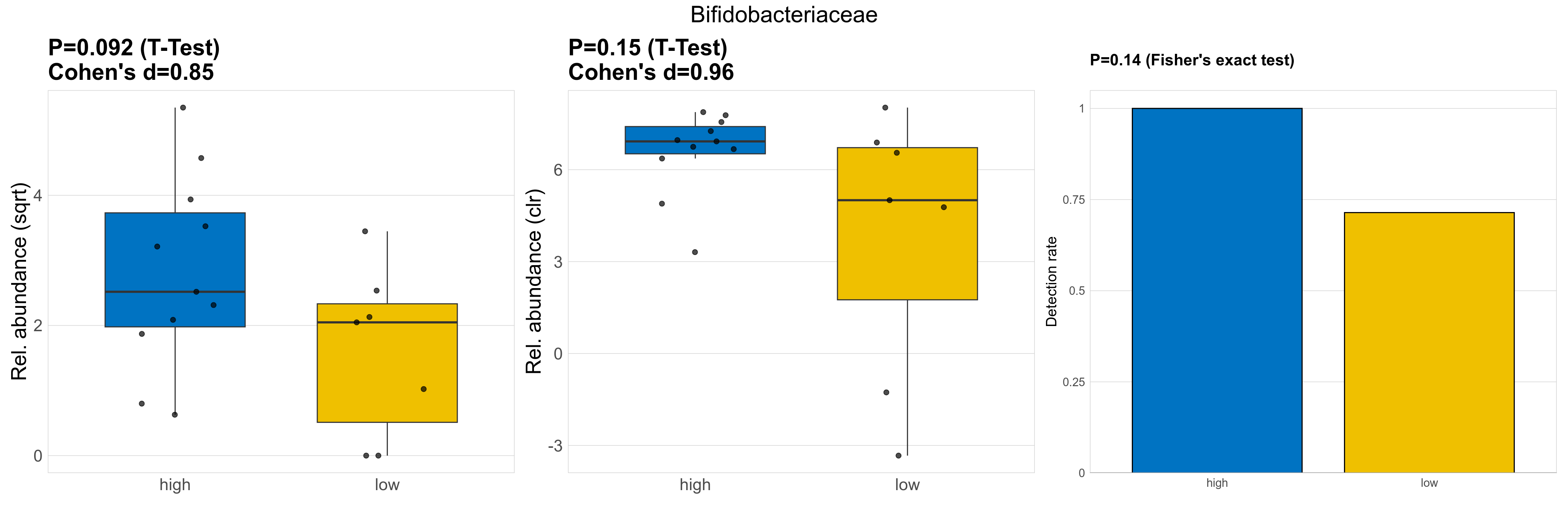
Bifidobacteriaceae	Bifidobacteriaceae	0.092	0.98	1	0.85	0.15	0.85	1	0.96	0.14	0.94	1	0.17	0.76	0.16	0.73	8.5	7.6	4.9	9.8	6.3	8.9	4	4.2	4.3	-1.3	16 / 18 (89%)	11 / 11 (100%)	5 / 7 (71%)	1	0.714
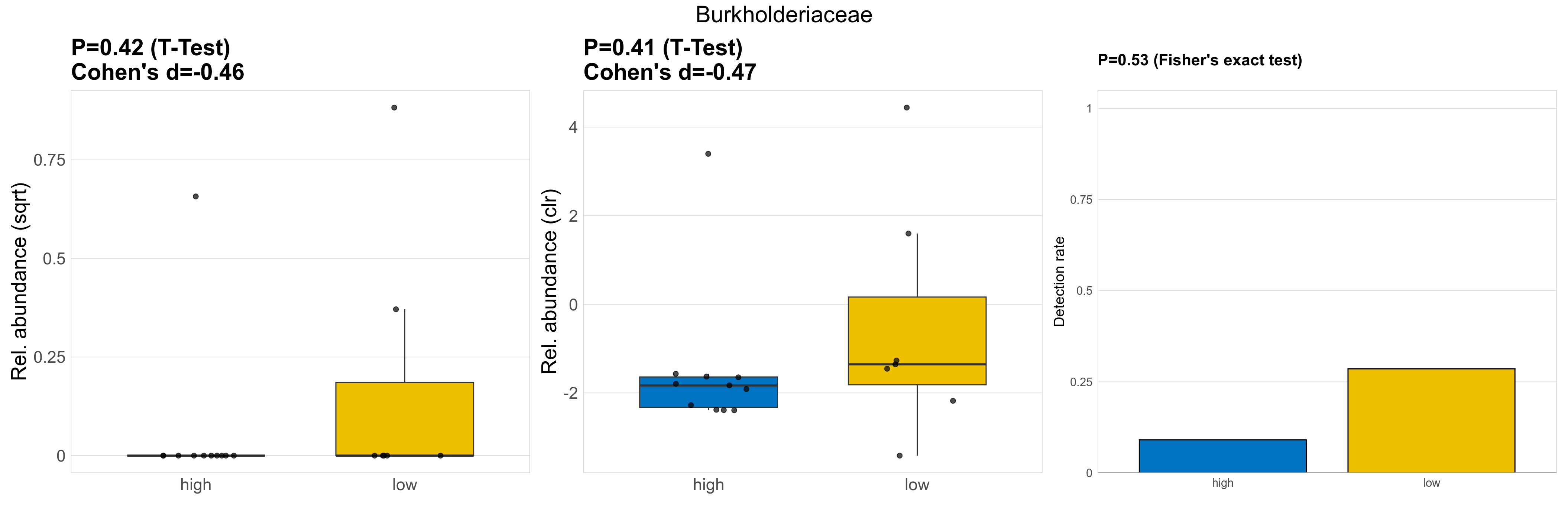
Burkholderiaceae	Burkholderiaceae	0.42	0.98	1	-0.46	0.41	0.85	1	-0.47	0.53	0.94	1	0.42	0.8	0.42	0.81	0.45	0.075	0	0.039	0	0.13	0.13	0	0.29	1.7	3 / 18 (17%)	1 / 11 (9.1%)	2 / 7 (29%)	0.0909	0.286
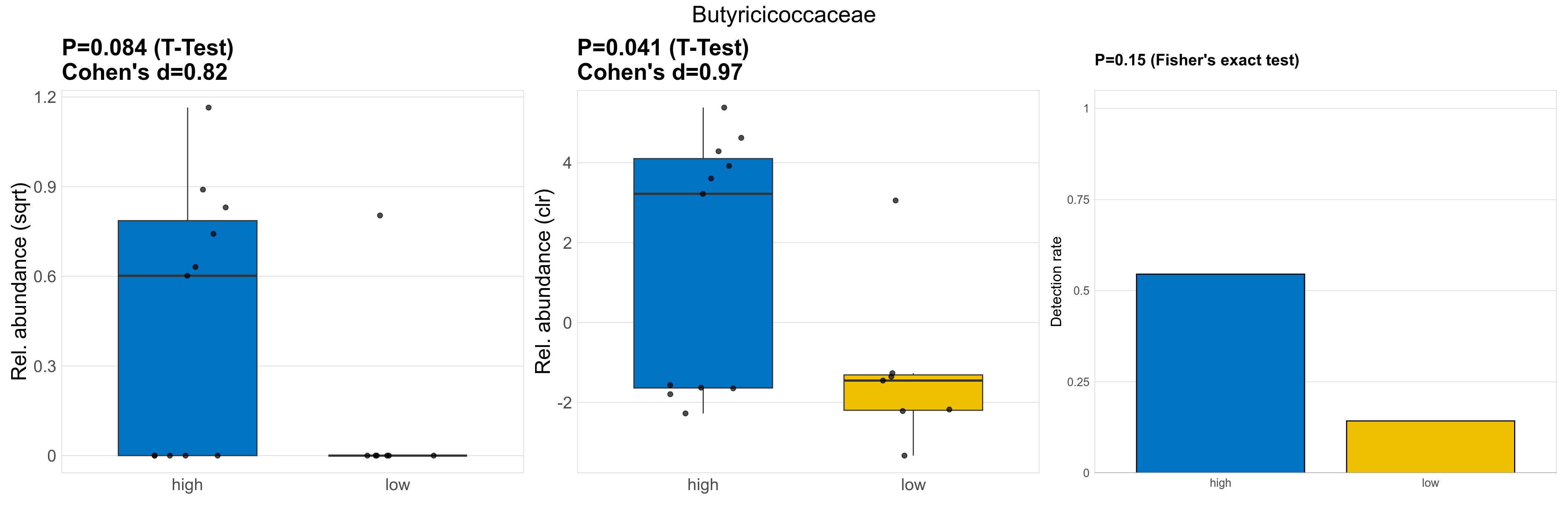
Butyricicoccaceae	Butyricicoccaceae	0.084	0.98	1	0.82	0.041	0.85	1	0.97	0.15	0.94	1	0.083	0.75	0.12	0.68	0.69	0.27	0	0.38	0.36	0.44	0.092	0	0.24	-2	7 / 18 (39%)	6 / 11 (55%)	1 / 7 (14%)	0.545	0.143
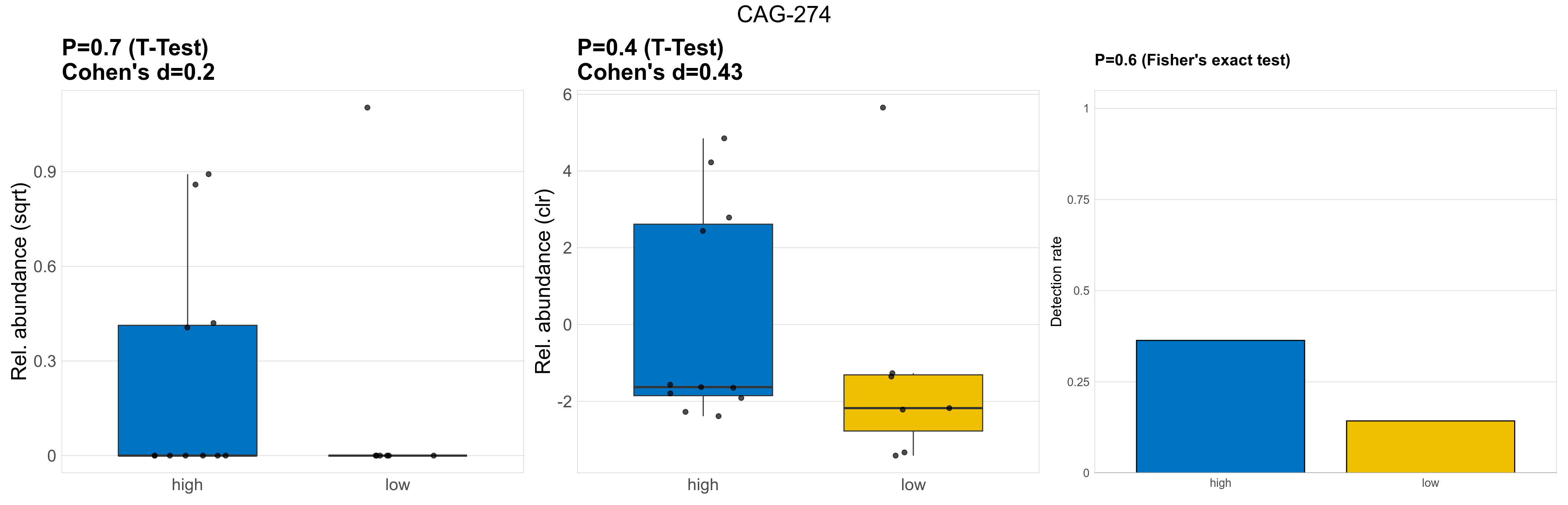
CAG-274	CAG-274	0.7	0.98	1	0.2	0.4	0.85	1	0.43	0.6	0.94	1	0.34	0.78	0.36	0.79	0.62	0.17	0	0.17	0	0.3	0.17	0	0.46	0	5 / 18 (28%)	4 / 11 (36%)	1 / 7 (14%)	0.364	0.143
CAG-302	CAG-302	0.63	0.98	1	0.22	0.67	0.89	1	0.19	1	1	1	0.71	0.89	0.7	0.93	0.62	0.1	0	0.13	0	0.3	0.054	0	0.14	-1.3	3 / 18 (17%)	2 / 11 (18%)	1 / 7 (14%)	0.182	0.143
CAG-508	CAG-508	0.66	0.98	1	0.21	0.65	0.89	1	0.22	1	1	1	0.67	0.87	0.74	0.94	0.58	0.19	0	0.23	0	0.46	0.13	0	0.25	-0.82	6 / 18 (33%)	4 / 11 (36%)	2 / 7 (29%)	0.364	0.286
CAG-74	CAG-74	0.74	0.98	1	-0.19	0.9	0.95	1	0.059	1	1	1	0.73	0.89	0.67	0.92	1.1	0.18	0	0.1	0	0.28	0.31	0	0.81	1.6	3 / 18 (17%)	2 / 11 (18%)	1 / 7 (14%)	0.182	0.143
Clostridiaceae	Clostridiaceae	0.86	0.98	1	0.083	0.85	0.95	1	0.086	1	1	1	0.76	0.9	0.71	0.93	0.31	0.087	0	0.095	0	0.18	0.074	0	0.16	-0.36	5 / 18 (28%)	3 / 11 (27%)	2 / 7 (29%)	0.273	0.286
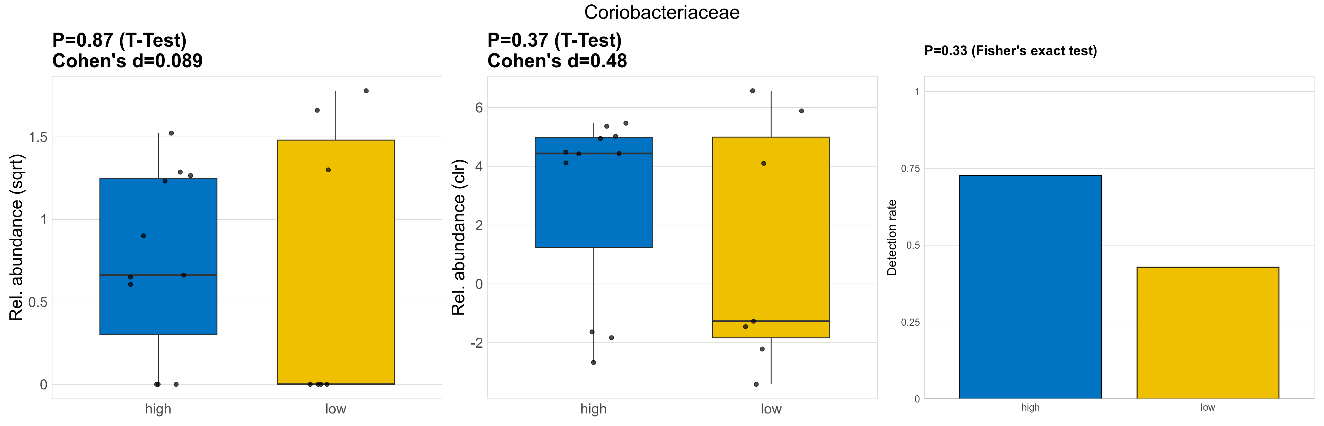
Coriobacteriaceae	Coriobacteriaceae	0.87	0.98	1	0.089	0.37	0.85	1	0.48	0.33	0.94	1	0.29	0.77	0.4	0.84	1.5	0.93	0.43	0.83	0.44	0.81	1.1	0	1.4	0.41	11 / 18 (61%)	8 / 11 (73%)	3 / 7 (43%)	0.727	0.429
Dialisteraceae	Dialisteraceae	0.83	0.98	1	-0.11	0.88	0.95	1	-0.079	1	1	1	0.86	0.93	0.81	0.95	1.3	0.51	0	0.48	0	0.83	0.57	0	1	0.25	7 / 18 (39%)	4 / 11 (36%)	3 / 7 (43%)	0.364	0.429
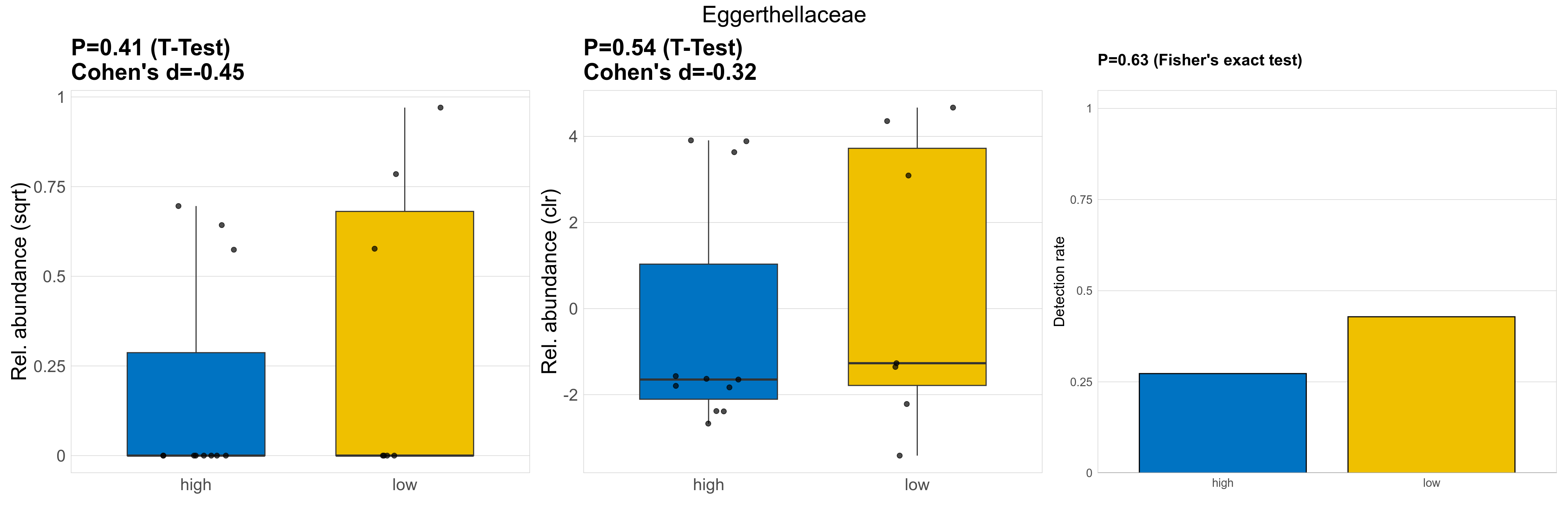
Eggerthellaceae	Eggerthellaceae	0.41	0.98	1	-0.45	0.54	0.86	1	-0.32	0.63	0.94	1	0.59	0.85	0.62	0.9	0.52	0.17	0	0.11	0	0.19	0.27	0	0.38	1.3	6 / 18 (33%)	3 / 11 (27%)	3 / 7 (43%)	0.273	0.429
Erysipelatoclostridiaceae	Erysipelatoclostridiaceae	0.99	0.99	1	0.0044	0.91	0.95	1	0.058	1	1	1	0.82	0.92	0.94	0.98	1	0.74	0.45	0.74	0.46	0.94	0.75	0.43	0.98	0.019	13 / 18 (72%)	8 / 11 (73%)	5 / 7 (71%)	0.727	0.714
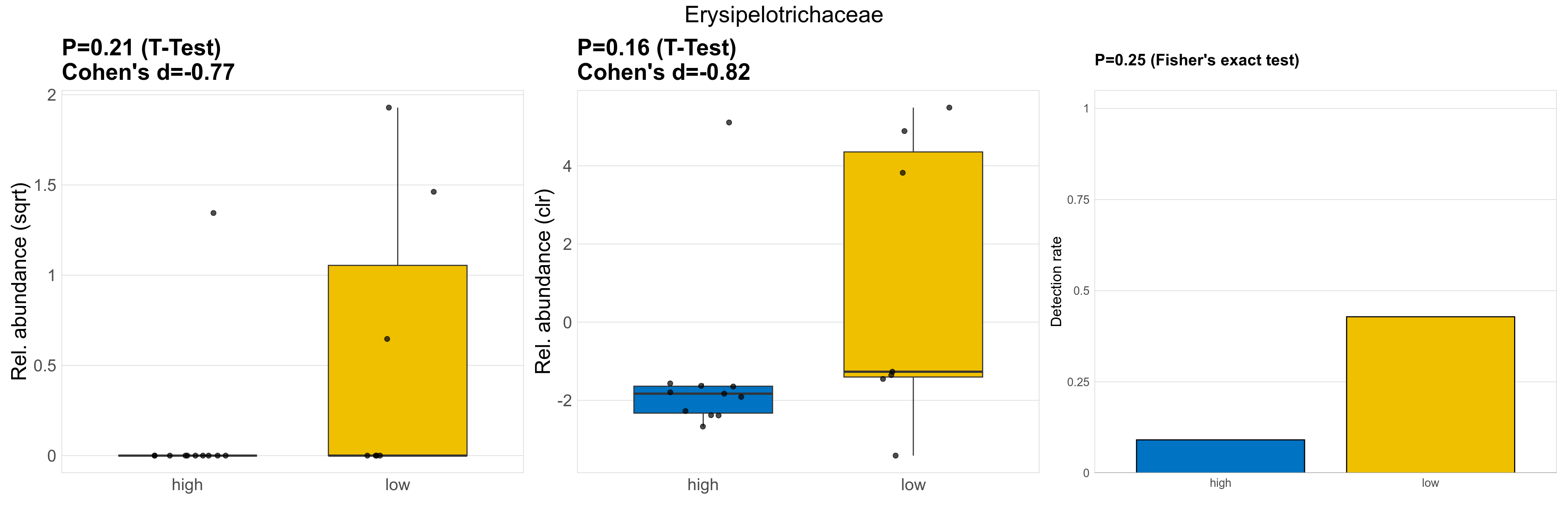
Erysipelotrichaceae	Erysipelotrichaceae	0.21	0.98	1	-0.77	0.16	0.85	1	-0.82	0.25	0.94	1	0.18	0.76	0.24	0.75	2	0.45	0	0.16	0	0.55	0.9	0	1.5	2.5	4 / 18 (22%)	1 / 11 (9.1%)	3 / 7 (43%)	0.0909	0.429
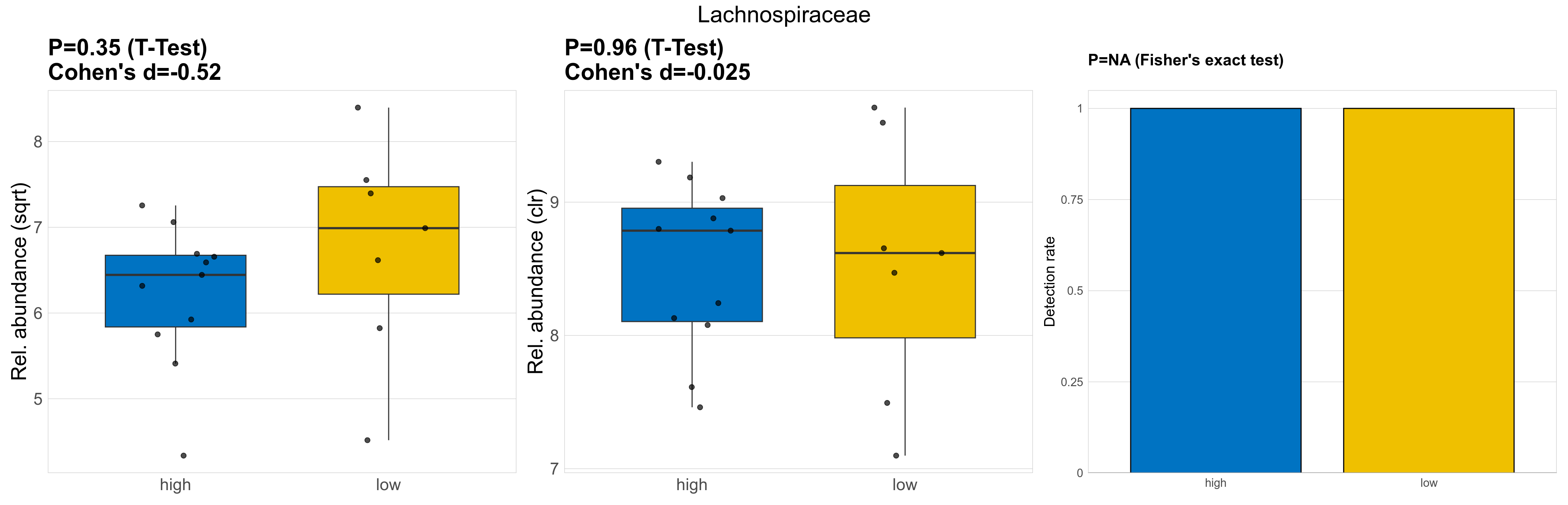
Lachnospiraceae	Lachnospiraceae	0.35	0.98	1	-0.52	0.96	0.96	1	-0.025	NA	NA	NA	0.77	0.91	0.88	0.97	42	42	44	39	42	9.7	47	49	16	0.27	18 / 18 (100%)	11 / 11 (100%)	7 / 7 (100%)	1	1
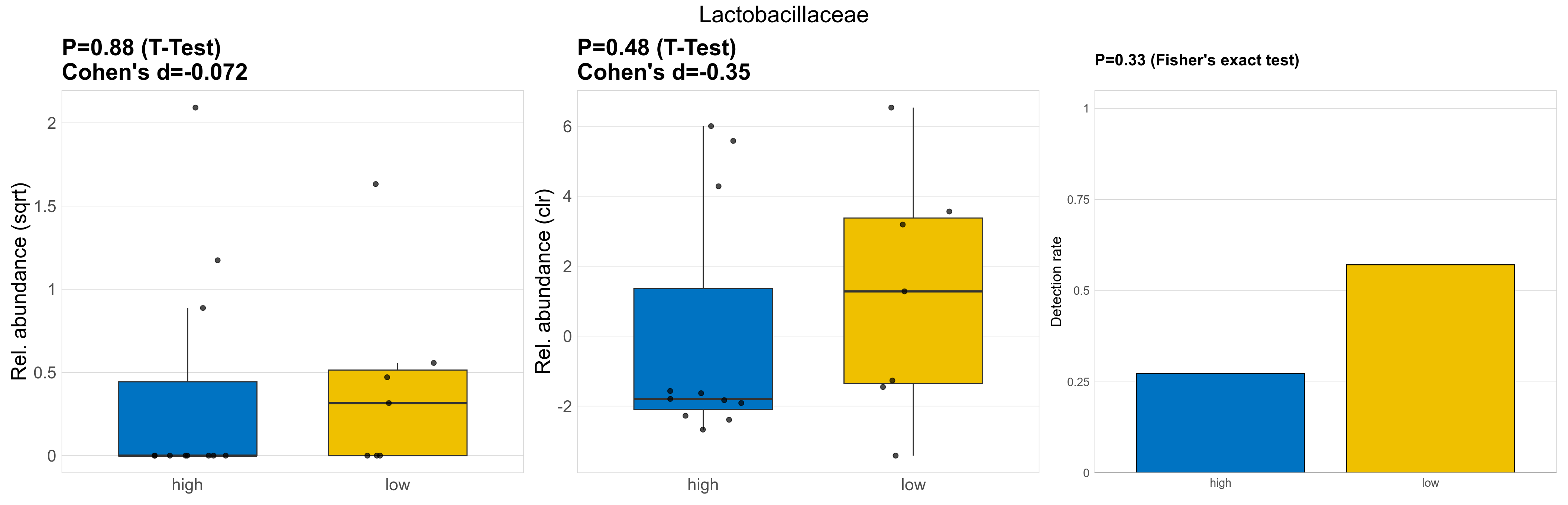
Lactobacillaceae	Lactobacillaceae	0.88	0.98	1	-0.072	0.48	0.85	1	-0.35	0.33	0.94	1	0.43	0.8	0.46	0.86	1.4	0.55	0	0.59	0	1.3	0.47	0.1	0.97	-0.33	7 / 18 (39%)	3 / 11 (27%)	4 / 7 (57%)	0.273	0.571
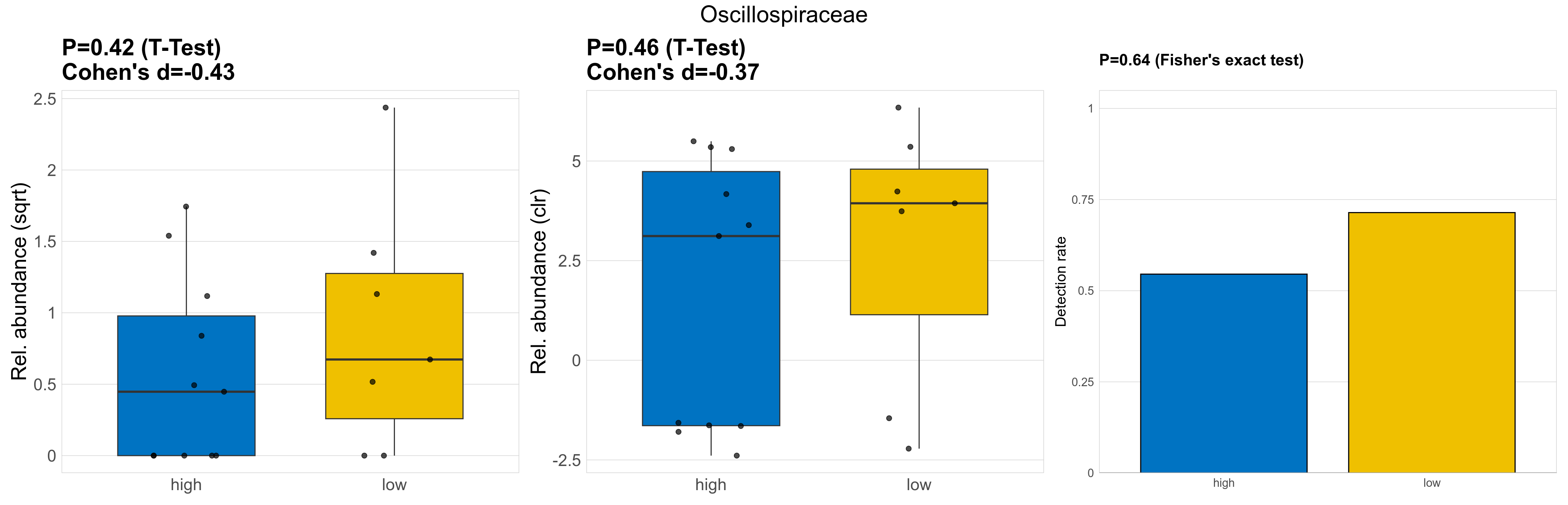
Oscillospiraceae	Oscillospiraceae	0.42	0.98	1	-0.43	0.46	0.85	1	-0.37	0.64	0.94	1	0.53	0.84	0.68	0.93	1.6	0.99	0.26	0.71	0.2	1.1	1.4	0.45	2.1	0.98	11 / 18 (61%)	6 / 11 (55%)	5 / 7 (71%)	0.545	0.714
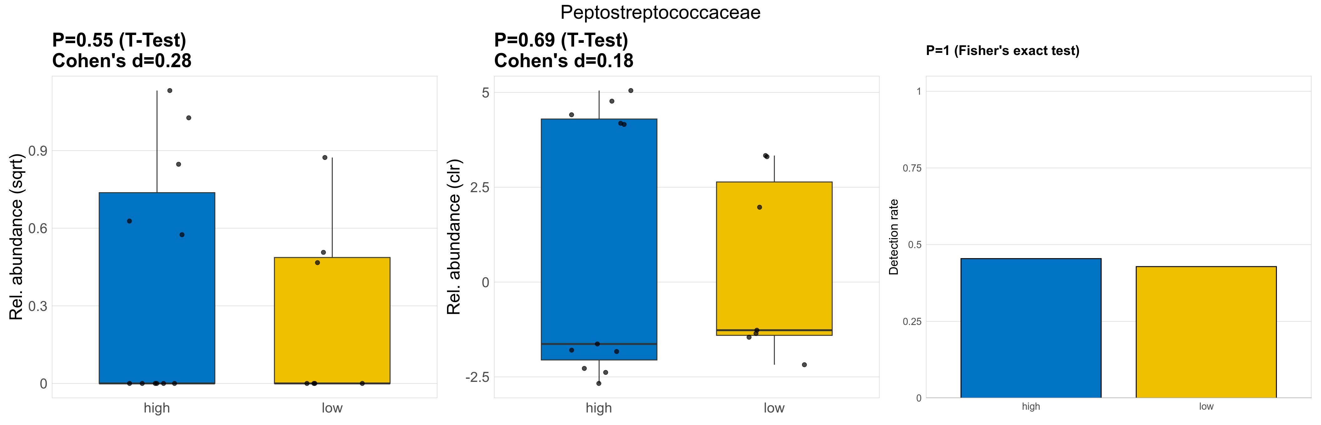
Peptostreptococcaceae	Peptostreptococcaceae	0.55	0.98	1	0.28	0.69	0.89	1	0.18	1	1	1	0.77	0.9	0.71	0.93	0.63	0.28	0	0.34	0	0.47	0.18	0	0.28	-0.92	8 / 18 (44%)	5 / 11 (45%)	3 / 7 (43%)	0.455	0.429
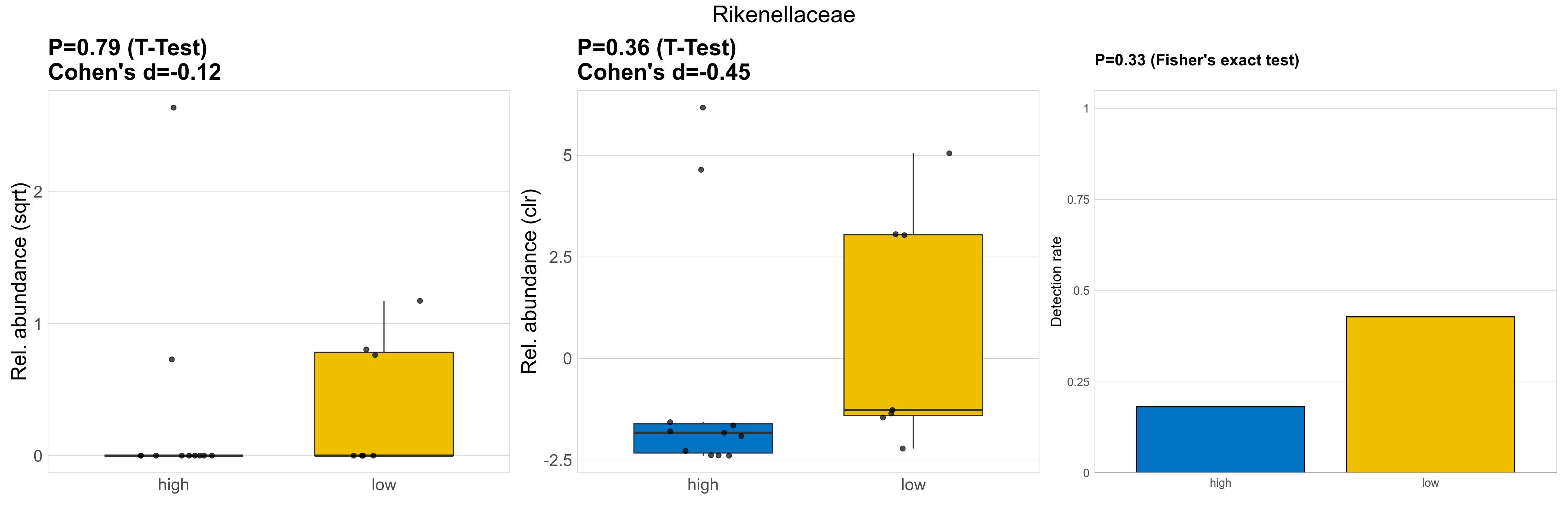
Rikenellaceae	Rikenellaceae	0.79	0.98	1	-0.12	0.36	0.85	1	-0.45	0.33	0.94	1	0.3	0.78	0.31	0.78	2	0.56	0	0.68	0	2.1	0.37	0	0.53	-0.88	5 / 18 (28%)	2 / 11 (18%)	3 / 7 (43%)	0.182	0.429
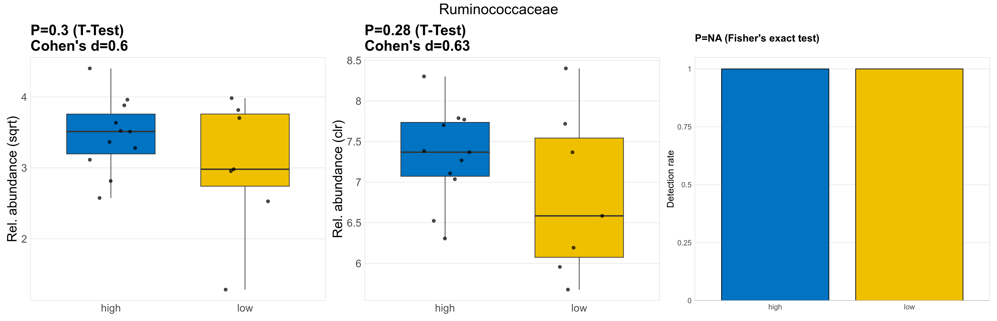
Ruminococcaceae	Ruminococcaceae	0.3	0.98	1	0.6	0.28	0.85	1	0.63	NA	NA	NA	0.31	0.77	0.29	0.8	11	11	12	12	12	3.6	10	8.9	5.1	-0.26	18 / 18 (100%)	11 / 11 (100%)	7 / 7 (100%)	1	1
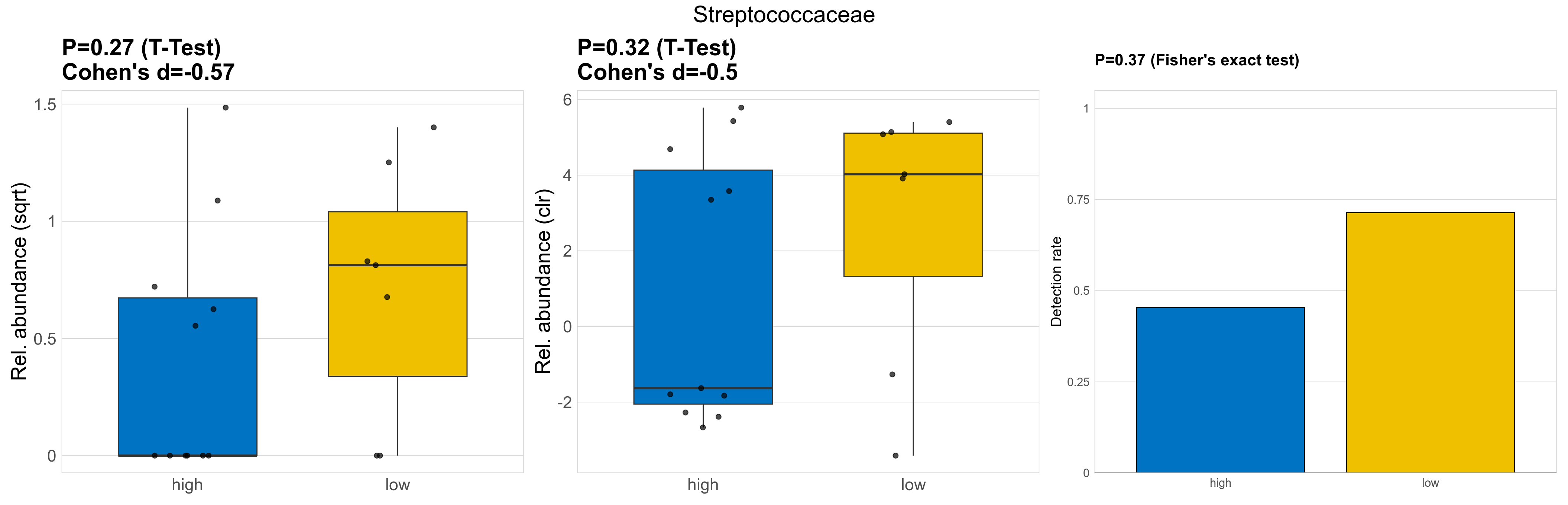
Streptococcaceae	Streptococcaceae	0.27	0.98	1	-0.57	0.32	0.85	1	-0.5	0.37	0.94	1	0.39	0.79	0.52	0.88	0.99	0.55	0.35	0.42	0	0.7	0.76	0.66	0.75	0.86	10 / 18 (56%)	5 / 11 (45%)	5 / 7 (71%)	0.455	0.714
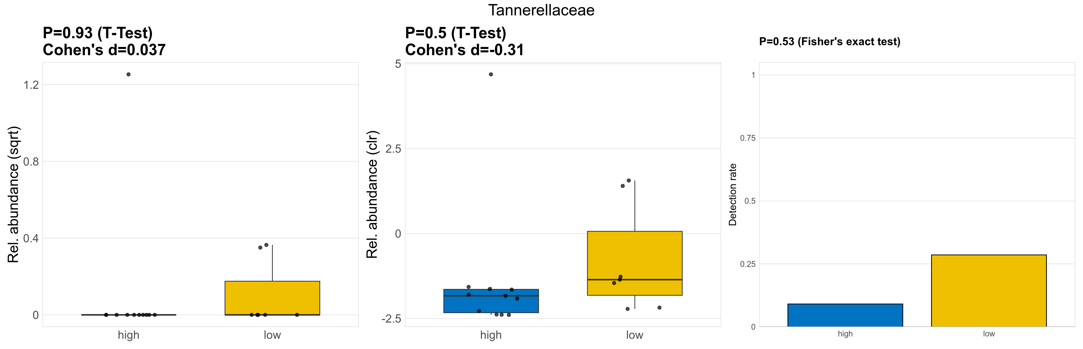
Tannerellaceae	Tannerellaceae	0.93	0.98	1	0.037	0.5	0.85	1	-0.31	0.53	0.94	1	0.45	0.82	0.41	0.82	0.61	0.1	0	0.14	0	0.47	0.037	0	0.062	-1.9	3 / 18 (17%)	1 / 11 (9.1%)	2 / 7 (29%)	0.0909	0.286
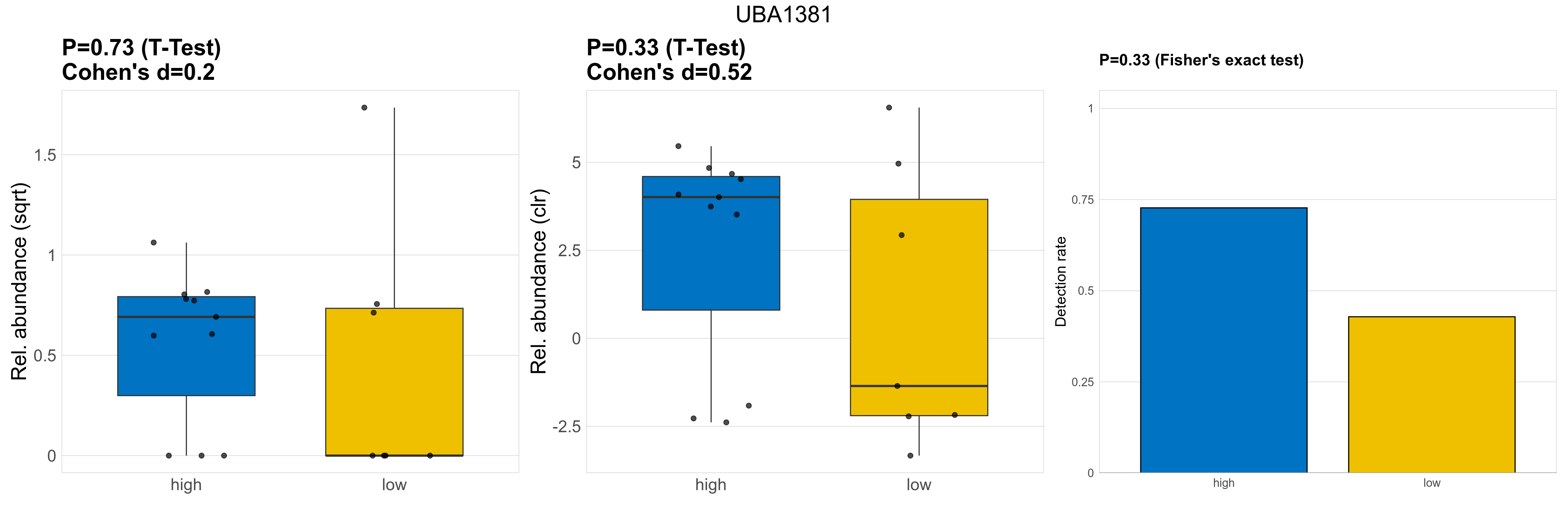
UBA1381	UBA1381	0.73	0.98	1	0.2	0.33	0.85	1	0.52	0.33	0.94	1	0.33	0.77	0.52	0.88	0.81	0.5	0.42	0.44	0.48	0.35	0.58	0	1.1	0.4	11 / 18 (61%)	8 / 11 (73%)	3 / 7 (43%)	0.727	0.429

Click here to open full-sized image in new window.

Click here to open full-sized image in new window.

Click here to open full-sized image in new window.

Click here to open full-sized image in new window.

Click here to open full-sized image in new window.

Methods:

P Fisher's exact test: differences in detection rate were detected by Fisher's exact test.

P Welch's t-test (sqrt): Differentially abundant species were identified by Welch's t-test.

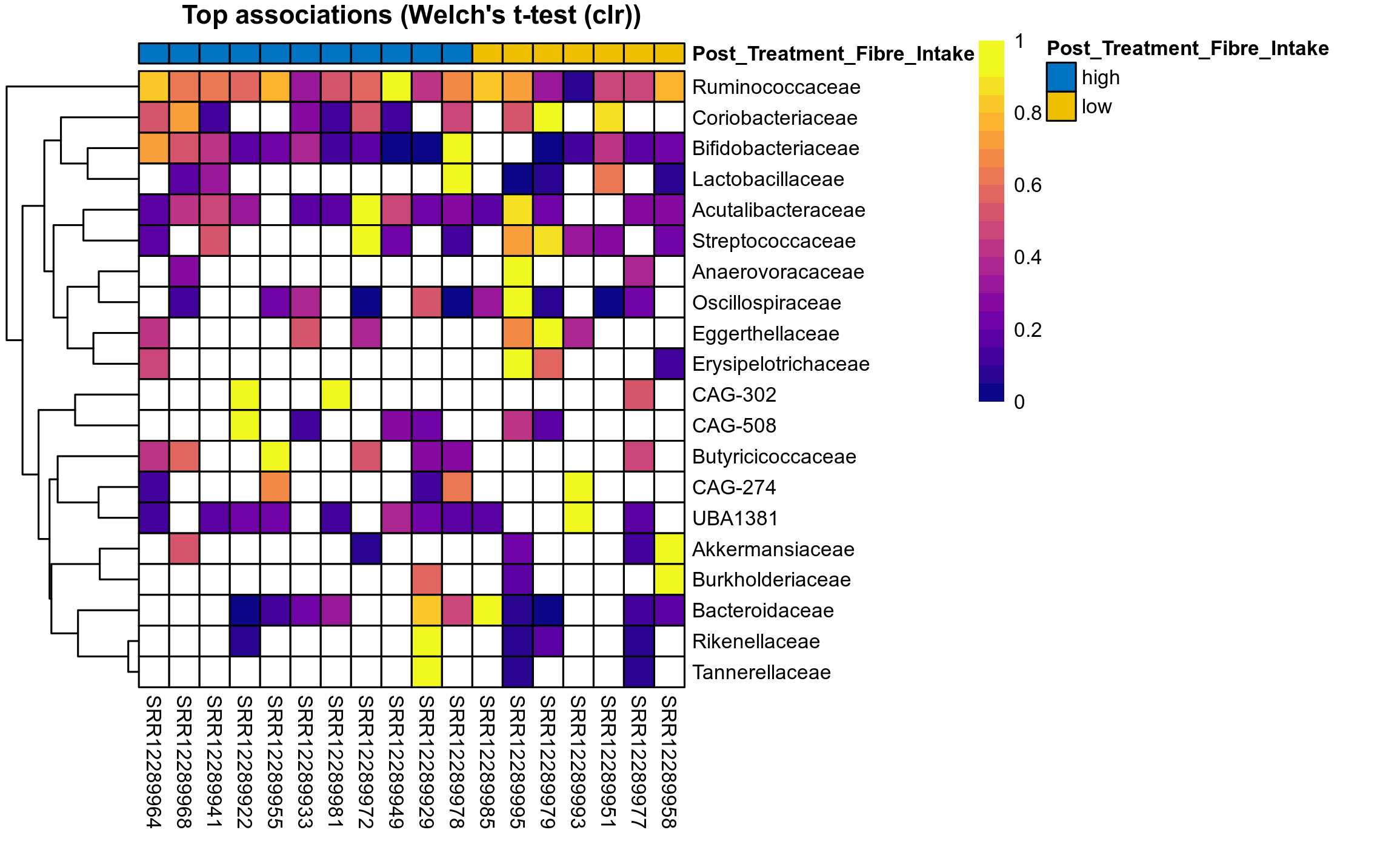
P Welch's t-test (clr): Differentially abundant species were identified by Welch's t-test.

Glossary:

clr: Centered log-ratio transformation. P Welch's ANOVA (sqrt): Welch's ANOVA p-values (Anova was run on sqrt transformed abundances). It is an alternative to the classic ANOVA and can be used even if the samples have unequal variances and/or unequal sample sizes. P Welch's t-test (sqrt): Welch's T-test p-values (run on sqrt transformed abundances). It is an alternative to the classic Student's t-test and is more reliable if the data violates the assumption of homogeneity of variances and/or if the study conditions have unequal sample sizes. P Welch's ANOVA (clr): Welch's ANOVA p-values (Anova was run on clr transformed abundances). It is an alternative to the classic ANOVA and can be used even if the samples have unequal variances and/or unequal sample sizes. P Welch's t-test (clr): Welch's T-test p-values (run on clr transformed abundances). It is an alternative to the classic Student's t-test and is more reliable if the data violates the assumption of homogeneity of variances and/or if the study conditions have unequal sample sizes. P lmer XXX (clr): P-value of Linear Mixed-Effects Regression on clr transformed abundances, testing significance of XXX effect. Varying intercepts per subjects are used to control for repeated measures. Pbonf: Bonferroni corrected p-value. FDR: False Discovery Rate q-value. Mean Pos: Mean abundance in positive samples. Positive samples: The number and percentage of samples in which each family has been detected. Positive XXX: The number and percentage of positive samples in study group XXX. Positive_XXX_percent: Percentage of positive samples in study group XXX. P Welch's t-test (Aldex2): Expected P value of Welch’s t-test computed by Aldex2. FDR Welch's t-test (Aldex2): Expected Benjamini-Hochberg corrected P value for Welch’s t-test. P Wilcoxon rank test (Aldex2): Expected P value of Wilcoxon rank test computed by Aldex2. FDR Wilcoxon rank test (Aldex2): Expected Benjamini-Hochberg corrected P value of Wilcoxon test. P Kruskal-Wallace test (Aldex2): Expected P value of Kruskal-Wallace test. FDR Kruskal-Wallace test (Aldex2): Expected Benjamini-Hochberg corrected P value of Kruskal-Wallace test. P GLM test (Aldex2): Expected P value of generalized linear model. FDR GLM test (Aldex2): Expected Benjamini-Hochberg corrected P value of generalized linear model.

Differentially abundant taxa (family)

The following plots present the distribution of the top most differentially abundant families across all applied statistical analysis. Plots are ordered alphabetically.

Glossary:

"Rel. Abundance": Relative abundance data; "Rel. Abundance (sqrt)": sqrt (Hellinger) transformed relative abundances; "Rel. Abundance (clr)": centered log-ratio (clr) transformed read counts.